Last year, Jordan Sellers and I published an article in Modern Language Quarterly, trying to trace the “great divide” that is supposed to open up between mass culture and advanced literary taste around the beginning of the twentieth century.
I’m borrowing the phrase “great divide” from Andreas Huyssen, but he’s not the only person to describe the phenomenon. Whether we explain it neutrally as a consequence of widespread literacy, or more skeptically as the rise of a “culture industry,” literary historians widely agree that popularity and prestige parted company in the twentieth century. So we were surprised not to be able to measure the widening gap.
We could certainly model literary taste. We trained a model to distinguish poets reviewed in elite literary magazines from a less celebrated “contrast group” selected randomly. The model achieved roughly 79% accuracy, 1820-1919, and the stability of the model itself raised interesting questions. But we didn’t find that the model’s accuracy increased across time in the way we would have expected in a period when elite and popular literary taste are specializing and growing apart.
Instead of concluding that the division never happened, we guessed that we had misunderstood it or looked in the wrong place. Algee-Hewitt and McGurl have pretty decisively confirmed that a divide exists in the twentieth century. So we ought to be able to see it emerging. Maybe we needed to reach further into the twentieth century — or maybe we would have better luck with fiction, since the history of fiction provides evidence about sales, as well as prestige?
In fact, getting evidence about that second, economic axis seems to be the key. It took work by many hands over a couple of years: Kyle Johnston, Sabrina Lee, and Jessica Mercado, as well as Jordan Sellers, have all contributed to this project. I’m presenting a preliminary account of our results at Cultural Analytics 2017, and this blog post is just a brief summary of the main point.
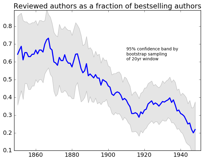
When you look at the books described as bestsellers by Publisher’s Weekly, or by book historians (see references to Altick, Bloom, Hackett, Leavis, below) it’s easy to see the two circles of the Venn diagram pulling apart: on the one hand bestsellers, on the other hand books reviewed in elite venues. (For our definition of “elite venues” see the “Table” in a supporting code & data repository.)
On the other hand, when you back up from bestsellers to look at a broader sample of literary production, it’s still not easy to detect increasing stylistic differentiation between the elite “reviewed” texts and the rest of the literary field. A classifier trained on the reviewed fiction has roughly 72.5% accuracy from 1850 to 1949; if you break the century into parts, there are some variations in accuracy, but no consistent pattern. (In a subsequent blog post, I’ll look at the fiddly details of algorithm choice and feature engineering, but the long and short of that question is — it doesn’t make a significant difference.)
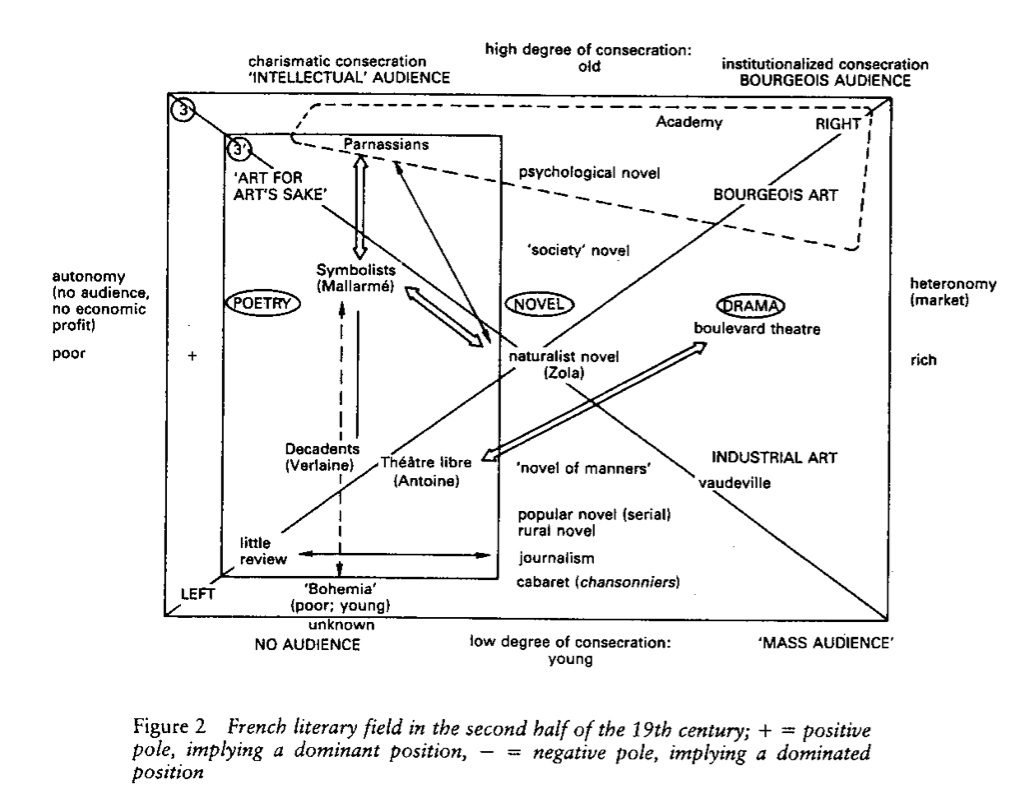
To understand why the growing separation of bestsellers from “reviewed” texts at the high end of the market doesn’t seem to make literary production as a whole more strongly stratified, I’ve tried mapping authors onto a two-dimensional model of the literary field, intended to echo Pierre Bourdieu’s well-known diagrams of the interaction between economic and cultural distinction.
Pierre Bourdieu, The Field of Cultural Production (1993), p. 49.
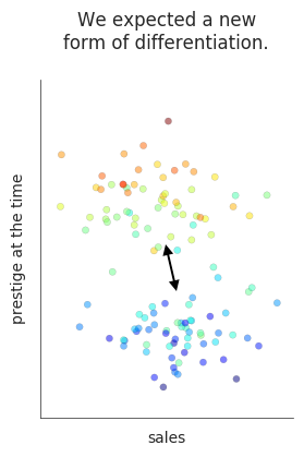
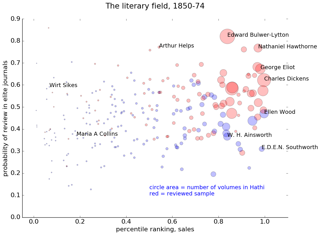
In the diagram below, for instance, the horizontal axis represents sales, and the vertical axis represents prestige. Sales would be easy to measure, if we had all the data. We actually don’t — so see the end of this post for the estimation strategy I adopted. Prestige, on the other hand, is difficult to measure: it’s perspectival and complex. So we modeled prestige by sampling texts that were reviewed in prominent literary magazines, and then training a model that used textual cues to predict the probability that any given book came from the “reviewed” set. An author’s prestige in this diagram is simply the average probability of review for their books. (The Stanford Literary Lab has similarly recreated Bourdieu’s model of distinction in their pamphlet “Canon/Archive,” using academic citations as a measure of prestige.)
The upward drift of these points reveals a fairly strong correlation between prestige and sales. It is possible to find a few high-selling authors who are predicted to lack critical prestige — notably, for instance, the historical novelist W. H. Ainsworth and the sensation novelist Ellen Wood, author of East Lynne. It’s harder to find authors who have prestige but no sales: there’s not much in the northwest corner of the map. Arthur Helps, a Cambridge Apostle, is a fairly lonely figure.
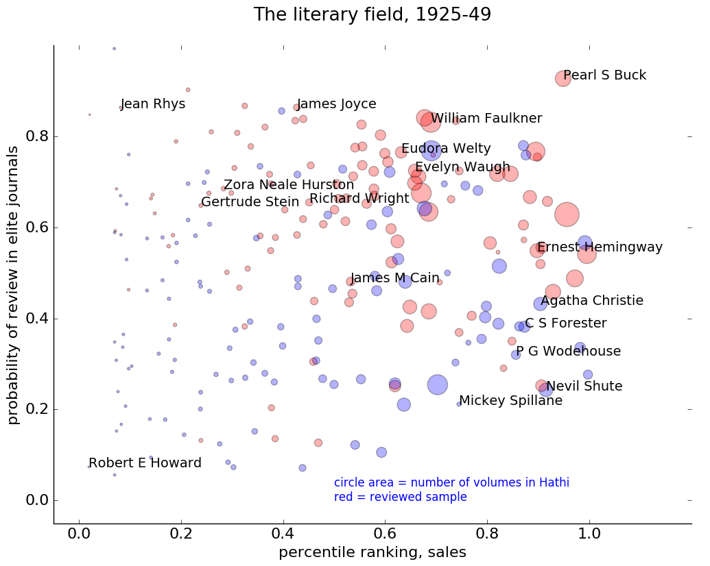
Fast-forward seventy-five years and we see a different picture.
The correlation between sales and prestige is now weaker; the cloud of authors is “rounder” overall.
There are also more authors in the “upper midwest” portion of the map now — people like Zora Neale Hurston and James Joyce, who have critical prestige but not enormous sales (or not up to 1949, at least as far as my model is aware).
There’s also a distinct “genre fiction” and “pulp fiction” world emerging in the southeast corner of this map, ranging from Agatha Christie to Mickey Spillane. (A few years earlier, Edgar Rice Burroughs and Zane Gray are in the same region.)
Moreover, if you just look at the large circles (the authors we’re most likely to remember), you can start to see how people in this period might get the idea that sales are actually negatively correlated with critical prestige. The right side of the map almost looks like a diagonal line slanting down from William Faulkner to P. G. Wodehouse.
That negative correlation doesn’t really characterize the field as a whole. Critical prestige still has a faint positive correlation with sales, as people over on the left side of the map might sadly remind us. But a brief survey of familiar names could give you the opposite impression.
In short, we’re not necessarily seeing a stronger stratification of the literary field. The change might better be described as a decline in the correlation of two existing forms of distinction. And as they become less correlated, the difference between them becomes more visible, especially among the well-known names on the right side of the map.
So, while we’re broadly confirming an existing story about literary history, the evidence also suggests that the metaphor of a “great divide” is a bit of an exaggeration. We don’t see any chasm emerging.
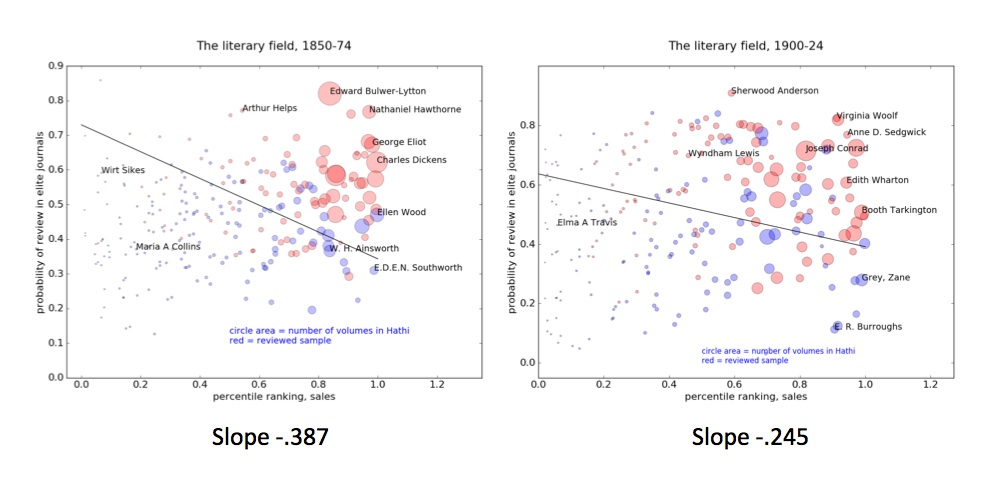
Maps of the literary field also help me understand why a classifier trained on an elite “reviewed” sample didn’t necessarily get stronger over time. The correlation of prestige and sales in the Victorian era means that the line separating the red and blue samples was strongly tilted there, and may borrow some of its strength from both axes. (It’s really a boundary between the prominent and the obscure.)
As we move into the twentieth century, the slope of the line gets flatter, and we get closer to a “pure” model of prestige (as distinguished from sales). But the boundary itself may not grow more clearly marked, if you’re sampling a group of the same size. (However, if you leave The New Republic and New Yorker behind, and sample only works reviewed in little magazines, you do get a more tightly unified group of texts that can be distinguished from a random sample with 83% accuracy.)
This is all great, you say — but how exactly are you “estimating” sales? We don’t actually have good sales figures for every author in HathiTrust Digital Library; we have fairly patchy records that depend on individual publishers.
For the answer to that question, I’m going to refer you to the github repo where I work out a model of sales. The short version is that I borrow a version of “empirical Bayes” from Julia Silge and David Robinson, and apply it to evidence drawn from bestseller lists as well as digital libraries, to construct a rough estimate of each author’s relative prominence in the market. The trick is, basically, to use the evidence we have to construct an estimate of our uncertainty, and then use our uncertainty to revise the evidence. The picture on the left gives you a rough sense of how that transformation works. I think empirical Bayes may turn out to be useful for a lot of problems where historians need to reconstruct evidence that is patchy or missing in the historical record, but the details are too much to explain here; see Silge’s post and my Jupyter notebook.
Bubble charts invite mouse-over exploration. I can’t easily embed interactive viz in this blog, but here are a few links to plotly visualizations:
The texts used here are drawn from HathiTrust via the HathiTrust Research Center. Parts of the research were funded by the Andrew G Mellon Foundation via the WCSA+DC grant, and part by SSHRC via NovelTM.
Most importantly, I want to acknowledge my collaborators on this project, Kyle Johnston, Sabrina Lee, Jessica Mercado, and Jordan Sellers. They contributed a lot of intellectual depth to the project — for instance by doing research that helped us decide which periodicals should represent a given period of literary history.
Algee-Hewitt, Mark, Sarah Allison, Marissa Gemma, Ryan Heuser, Franco Moretti, Hannah Walser. “Canon/Archive: Large-Scale Dynamics in the Literary Field.” Stanford Literary Lab, January 2016. https://litlab.stanford.edu/LiteraryLabPamphlet11.pdf
Altick, Richard D. The English Common Reader: A Social History of the Mass Reading Public 1800-1900. Chicago: University of Chicago Press, 1957.
Bloom, Clive. Bestsellers: Popular Fiction Since 1900. 2nd edition. Houndmills: Palgrave Macmillan, 2008.
Hackett, Alice Payne, and James Henry Burke. 80 Years of Best Sellers 1895-1975. New York: R.R. Bowker, 1977.
Leavis, Q. D. Fiction and the Reading Public. 1935.
Mott, Frank Luther. Golden Multitudes: The Story of Bestsellers in the United States. New York: R. R. Bowker, 1947.
This year, we’re returning to that simple question, with a richer dataset (supported by ongoing work at HathiTrust Research Center). The full story will come out in an article, but we’d like to share a few big-picture points in advance.
To start with, why have we framed this as a question about “women” and “men”? Gender isn’t a binary phenomenon. But we aren’t inquiring about the truth of gender identity here — just about gross inequalities that have separated conventional public roles. English-language fiction does typically divide characters by calling them “he” or “she,” and that division is a good place to start posing questions.
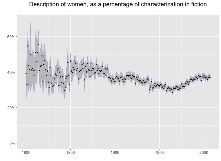
We could measure underrepresentation by counting people, but then we’d have to decide how much weight to give minor characters. A simpler approach is just to ask how many words are used to describe fictional men or women, respectively. BookNLP gave us a way to answer that question; it uses names and honorifics to infer a character’s gender, and then traces grammatical dependencies to identify adjectives that modify a character, nouns she possesses, or verbs she governs. After swinging BookNLP through 93,708 English-language volumes identified as fiction from the HathiTrust Digital Library, we can estimate the percentage of words used in characterization that are used to describe women. (To simplify the task of reading this illustration, we have left out characters coded as “other” or unknown,” so a year with equal representation of men and women would be located on the 50% line.). To help quantify our uncertainty, we present each measurement by year along with a 95% confidence interval calculated using the bootstrap; our uncertainty decreases over time, largely as a function of an increasing number of books being published.
There is a clear decline from the nineteenth century (when women generally take up 40% or more of the “character space” in fiction) to the 1950s and 60s, when their prominence hovers around a low of 30%. A correction, beginning in the 1970s, almost restores fiction to its nineteenth-century state. (One way of thinking about this: second-wave feminism was a desperately-needed rescue operation.)
The fluctuation is not enormous, but also not trivial: women lose roughly a fourth of the space on the page they had possessed in the nineteenth century. Nor is this something we already knew. It might be a mistake to call this pattern a “surprise”: it’s not as if everyone had clearly-formed expectations about “space on the page.” But when we do pose the question, and ask scholars what they expect to see before revealing this evidence, several people have predicted a series of advances toward equality that correspond to e.g. the suffrage movement and World War II, separated by partial retreats. Instead we see a fairly steady decline from 1860 to 1970, with no overall advance toward equality.
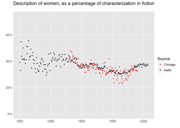
What’s the explanation? Our methods do have blind spots. For instance, we aren’t usually able to infer gender for first-person protagonists, so they are left out here. And our inferences about other characters have a known level of error. But after cross-checking the evidence, we don’t believe the level of error is large enough to explain away this pattern (see our github repo for fuller discussion). It is of course possible that our sample of fiction is skewed. For instance, a sample of 93,708 volumes will include a lot of obscure works and works in translation. What if we focus on slightly more prominent works? We have posed that question by comparing our Hathi sample to a smaller (10,000-volume) sample drawn from the Chicago Text Lab, which emphasizes relatively prominent American works, and filters out works in translation.
As you can see, the broad outlines of the trend don’t change. If anything, the decline from 1860 to 1970 is slightly more marked in the Chicago corpus (perhaps because it does a better job of filtering out reprints, which tend to muffle change). This doesn’t prove that we will see the same pattern in every sample. There are many ways to sample the history of fiction! Some scholars will want to know about paperbacks that tend to be underrepresented in university libraries; others will only be interested in a short list of hypercanonical authors. We can’t exhaust all possible modes of sampling, but we can say at least that this trend is not an artefact of a single sampling strategy. Nor is it an artefact of our choice to represent characters by counting words syntactically associated with them: we see the same pattern of decline to different degrees when measuring the amount of dialogue spoken by men and women, and in simply counting the number of characters as well.
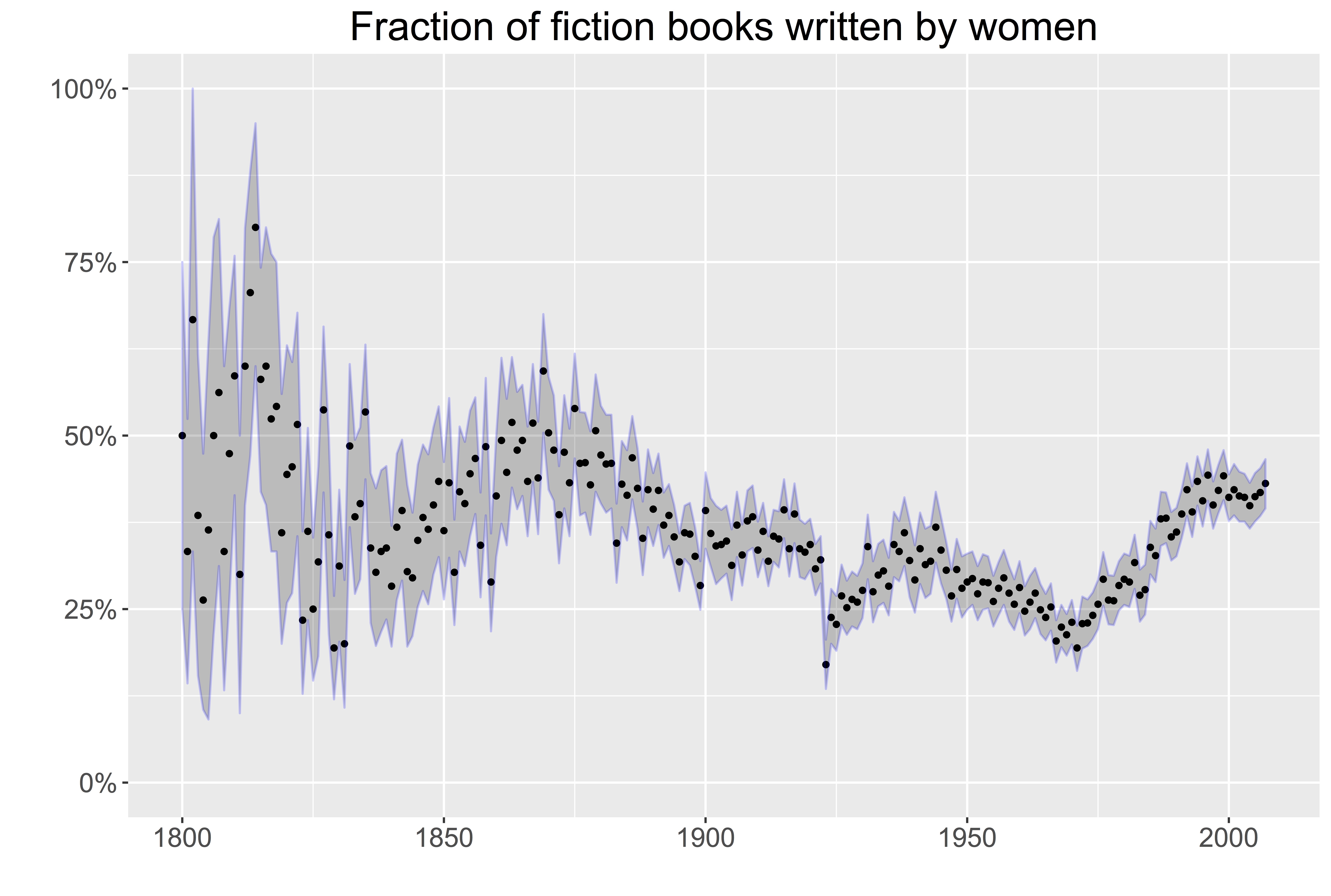
So what does explain the declining representation of women? We don’t yet know. But the trend seems too complex to dismiss with a single explanation. For instance, it can be partly — but only partly — explained by a decline in the proportion of fiction writers who were women.
Take specific dots with a grain of salt; there are sources of error here, especially because the wall of copyright at 1923 may change digitization practices or throw off our own data pipeline. (Note the outlier right at 1923.) But the general pattern above is echoed also in the Chicago sample of American fiction, so we feel confident that there was really a decline in the fraction of fiction writers who were women. As far as we know, Chris Forster was the first person to gather broad quantitative evidence of this decline. But many scholars have grasped pieces of the story: for instance, Anne E. Boyd takes The Atlantic around 1890 as a case study of a process whereby the professionalization and canonization of American fiction tended to push out women who had previously been prominent. [See also Tuchman and Fortin 1989 in references below.]
But this is not necessarily a story about the marginalization of women writers in general. (On the contrary, the prominence of women rose throughout this period in several nonfiction genres.) The decline was specific to fiction — either because the intellectual opportunities open to women were expanding beyond belles lettres, or because the rising prestige of fiction attracted a growing number of men.
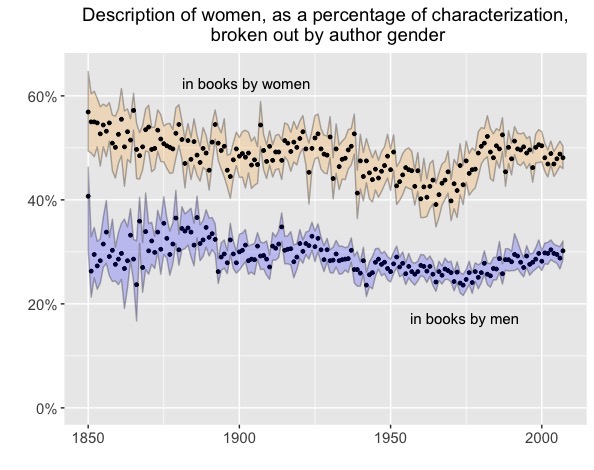
Men are overrepresented in books by men, so a decline in the number of women novelists will also tend to reduce the number of characters who are women. But that doesn’t completely explain the marginalization of feminine characters from 1860 to 1970. For instance, we can also divide authors by gender, and look at shifting patterns of attention within works by women or by men.
There are several interesting details here. The inequality of attention in books by men is depressingly durable (men rarely give more than 30% of their attention to fictional women). But it’s also interesting that the fluctuations we saw earlier remain visible even when works are divided by author gender: both trend lines above show a slight decline in the space allotted to women, from 1860 to 1970. In other words, it’s not just that there were fewer works of fiction written by women; even inside books written by women, feminine characters were occupying slightly less space on the page.
Why? The rise of genres devoted to “action” and “adventure” might play a role, although we haven’t found clear evidence yet that it makes a difference. (Genre boundaries are too blurry for the question to be answered easily.) Or fiction might have been masculinized in some broader sense, less tied to specific genre categories (see Suzanne Clark, for instance, on modernism as masculinization.)
But listing possible explanations is the easy part. Figuring out which are true — and to what extent — will be harder.
We will continue to explore these questions, in collaboration with grad students, but we also want to draw other scholars’ attention to resources that can support this kind of inquiry (and invite readers to share useful secondary sources in the comments).
When we publish our article, we will also share data produced by BookNLP about specific characters across a collection of 93,708 books. HTRC is also building a “Data Capsule” that will allow other scholars to produce similar data themselves. In the meantime, in collaboration with Nikolaus N. Parulian, we have produced an interactive visualization that allows you to explore changes in the gendering of words used in characterization. (Compare, for instance, “grin” to “smile,” or “house” to “room.”) We have also made available the metadata and yearly summaries behind the visualization.
Acknowledgments. The work described here has been supported by NovelTM, funded by the Canadian Social Sciences and Humanities Research Council, and by the WCSA+DC grant at HathiTrust Research Center, funded by the Andrew W. Mellon Foundation. We thank Hoyt Long, Teddy Roland, and Richard Jean So for permission to use the Chicago Novel Corpus. The project often relied on GenderID.py, by Bridget Baird and Cameron Blevins (2014). Boris Capitanu helped parallelize BookNLP across hundreds of thousands of volumes. Attendees at the 2016 NovelTM meeting, and Justine Murison in Illinois, provided valuable advice about literary history.
References.
Boyd, Anne E. “‘What, Has She Got into the Atlantic?’ Women Writers, The Atlantic Monthly, and the Formation of the American Canon,” American Studies 39.3 (1998): 5-36.
Clark, Suzanne. Sentimental Modernism: Women Writers and the Revolution of the Word (Indianapolis: Indiana University Press, 1992).
Literary critics have been having a speculative conversation about close and distant reading. It might be premature to call it a debate.
A “debate” is normally a situation where people are free to choose between two paths. “Should I believe Habermas, or Foucault? I’m listening; I could go either way.” Conversation about distant reading is different, first, because there’s not much need to make a choice. Have any critics stopped reading closely? A close reading of The Bourgeois suggests that Franco Moretti hasn’t.
More importantly, this isn’t a debate yet because most of the people involved aren’t free to explore both paths. So far only a tiny number of scholars have actually tried distant reading, and it’s easy to see why. You can wake up tomorrow and try a Foucauldian reading of Frankenstein, but you can’t wake up and trace patterns of change in a thousand novels. In either case, you may need to learn new methods, but in the “distant” case, it can also take years to assemble a collection of texts.
A dataset for distant reading
To reduce barriers to entry, I’ve collaborated with HathiTrust Research Center to create an easier place to start with English-language literature. It’s aimed at scholars studying long-nineteenth-century (1750-1922) fiction and poetry, but it will gradually expand into the twentieth century. This post describes the humanistic uses of the dataset; if you want technical information, there’s more on the page where the data actually lives.
HathiTrust contains more than a million volumes in English between 1700 and 1922. Contractual agreements make it hard to share the texts themselves in bulk, but many of the questions that can be posed “at a distance” can be posed just as well using simpler representations of the texts — for instance, by counting the words they contain. To support this project, HathiTrust Research Center has extracted page-level word counts for 4.8 million volumes; scholars who are interested in the highest level of detail should go directly to their data.
However, many literary scholars are mainly concerned with books in a particular genre — they limit their inquiries, say, to “poetry” or “prose fiction.” Finding those needles in a five-millon-volume haystack is not easy. Many books in this period don’t carry genre tags; even when they do, volumes are heterogenous things. A volume of poetry, for instance, may begin with a prose life of the author and end with publishers’ ads.
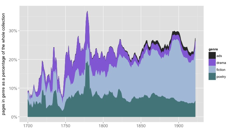
The relative sizes of different genres, represented as a percentage of pages in the English-language portion of HathiTrust. 854,476 volumes are covered. Nonfiction, front matter, and back matter aren’t represented here. Results have been smoothed with a five-year moving average.
To create datasets that reliably track a single genre, we need page-level metadata. The National Endowment for the Humanities and the American Council of Learned Societies funded a year-long project to create that metadata. (The methods involved are described in a white paper on “Understanding Genre,” along with information about accuracy.) Now, by pairing this metadata with HTRC’s page-level wordcounts, I’ve created three genre-specific datasets of word counts covering poetry, fiction, and drama from 1700 to 1922. (Coverage is relatively sparse before 1750; if you need the early eighteenth century, you might want a resource like ECCO-TCP instead of or in addition to this.)
The collection consists of word counts for 101,948 volumes of fiction, 58,724 volumes of poetry, and 17,709 volumes of drama, aggregated at the volume level and including only pages identified as belonging to the relevant genre. I’ve collected these volume-level files in tar.gz chunks by genre and date, and have provided basic metadata for them all. You can use the volume IDs to view the original texts on the HathiTrust website if you need to read them closely. I’m calling this a “collection” rather than a “corpus” because I don’t necessarily recommend that you use the whole thing, as is. The whole thing may or may not represent the sample you need for your research question. What it represents is, “American university and public libraries, insofar as they were digitized in the year 2012 (when the project began).” For some big diachronic questions, that’s a good sample; for other questions, you’ll need to be more selective.
Three big blocks of stone. Like collections, these don’t represent anything in particular. But like a statue, the corpus you want to create might be contained somewhere within them.
Because this is a very large collection, it’s likely in any case that the sample you need for your research may be contained somewhere within it. To address some questions, you might even select several samples and contrast them. To understand the history of literary prestige, for instance, Jordan Sellers and I gathered 360 prominent books of poetry by finding reviews in literary magazines and extracting the corresponding books from HathiTrust; we then contrasted that to a sample of 360 more obscure volumes selected from the whole HathiTrust collection of poetry. Just using volume-level wordcounts for those two samples, we were able to draw inferences about the way diachronic literary change is related to synchronic prestige.
Well-known texts may be represented in this dataset by dozens of reprints. For some questions, that may be exactly the sort of “weighted” sample you want; for other questions, you’ll want to winnow each title down to a single early example. More datasets may be developed to help you do that.
Distant reading rarely means “big data”
I realize the practice described above (selecting samples of a few hundred or a few thousand books to address particular questions) doesn’t line up with the version of distant reading currently circulating in public imagination. Isn’t the point of distant reading to construct a massive database that includes “everything that has been thought and said”?The Nation recently said so, and also warned us that “in reality, servers powerful enough to process big data can only be located in a highly select number of well-endowed institutions.”
That sounds grim, but I’m happy to report that it’s also malarkey. You can download this dataset, and process it, on your laptop. It’s true that I used our campus cluster to create it (because I had to manage a terabyte of text). But a) managing a terabyte won’t put a hole in most endowments, and b) you don’t need to do that anyway. Once nonfiction is set aside, we’re talking about a smaller group of books (compressed, this whole dataset runs to about 5GB). A well-designed sampling strategy can make it even smaller.
Wait, what’s this about “sampling”? aren’t distant readers supposed to claim to have everything? Not really. In the early days of distant reading, Franco Moretti did frame the project as a challenge to literary historians’ claims about synchronic coverage. (We only discuss a tiny number of books from any given period — what about all the rest?) But even in those early publications, Moretti acknowledged that we would only be able to represent “all the rest” through some kind of sample.
Fifteen years later, it’s becoming clear that distant reading has a lot of applications that aren’t about synchronic completeness at all. Expanding the diachronic scope of our research can be an equally important source of discovery. Certain kinds of change only become visible when you compare many examples across long timelines. Even if we restricted a digital corpus (say) to the academic canon, or to a thousand bestsellers, computational analysis would allow us to see long-term changes that aren’t visible to casual recollection.
It’s true that distant readers will often want to have the biggest possible table of metadata, so that our sampling strategies aren’t unduly constrained. But from that table, we may only sample a few hundred or a few thousand titles to address any single question. This scale of inquiry is not, in any meaningful sense, “big data.” (In fact, I doubt the phrase “big data” is often very meaningful, but that’s another story.) It’s a larger sample than literary scholars have usually attempted to describe, but it would not greatly distress our neighbors in linguistics and sociology.
How hard is this to use?
Of course, we’re not linguists or sociologists, so there is going to be a learning curve involved when we apply quantitative methods on any scale. The main dataset I’m providing here includes 178,381 separate files — one file for each volume. This is not something that can be sliced easily using a tool like Excel. Someone involved with the project needs to be able to program in order to pair the metadata table with the files.
On the other hand, there may be some questions that can be answered with a simple yearly summary, so I’ve also provided yearly_summary tables for each genre that aggregate term frequencies for the 10,000 most common tokens in each genre (selected by document frequency). This is the gentlest on-ramp to the dataset; data in this form probably can be sliced with Excel; to make it even easier I’ve also gone ahead and applied OCR correction and spelling normalization to those tables.
But the yearly_summary table aggregates all the volumes in the collection, and (as I’ve stressed) you may not want all of them. This dataset is a roughly-hewn, but very large, block of stone. You may be able to find the corpus you need somewhere within it, but decisions about selection are yours to make. Over the course of the next two years I hope to extend coverage further into the twentieth century; it is not illegal to share word counts from texts still covered by copyright. If you’re interested in more complex kinds of distant reading where word order matters, you can contact the HathiTrust Research Center; they are creating a workflow that can handle more complex kinds of computational analysis.
Postscript: We’ve done a lot of testing, but this is still a beta release. General estimates about error are summarized in “Understanding Genre”. Precision in these datasets is higher than 97%, but that still means there will be hundreds of volumes and thousands of pages mistakenly included. If you notice systematic problems with the data, please send feedback to the e-mail address provided in the data description. But individual misclassified volumes are not problems we’re likely to fix on a case-by-case basis; that sort of problem will be addressed by improving our methods in our next release.
Part of this project will appear next year — revised and improved — in MLQ. But we’ve decided to release it as a free-standing draft rather than a preprint, because it allows us to use color and to explore some puzzling leads that won’t fit into the physical limits of one journal article.
To understand the aesthetic standards that govern reception, we contrasted two samples of English-language poetry, drawn from different social contexts: 1) a group of 360 volumes that we chose by sampling reviews in prominent periodicals, 1820-1919, and 2) a group of 360 volumes sampled at random from HathiTrust Digital Library, many of them pretty obscure.
We were curious whether the difference in prestige between these books would be legible in the texts themselves. For instance, could you train a statistical model to predict whether a volume of poetry came from the “reviewed” or “random” sample just by looking at diction? And if you could, what social difference exactly would you be detecting?
Scholars sometimes suggest that high culture hadn’t differentiated from the rest of the literary field very sharply yet in the early 19th century [1: Huyssen 1986]. If so, books of poetry reviewed in prestigious contexts might be hard to identify in that part of the timeline. It might get easier toward the 20th century, as different poetic styles specialized to address (say) “high” and “middlebrow” audiences.
On the other hand, if writers became prominent by occupying the leading edge of a rapidly-moving wave, we might only be able to separate these samples by training a sequence of different models for different periods. For instance, prominent poets in the 1820s might be united by gloomy Byronism; in the 1850s they might share an interest in history; by the 1890s what they had in common might be the word “mauve.” As for the randomly-selected volumes, who knows? Maybe they would share only a tendency to trail thirty years behind the trend.
Since it seemed reasonable to assume that the standards governing reception had been volatile, we began by training a different model of poetic prestige for each twenty-year period. But we found, in practice, that the best way to separate these samples was to treat the whole period 1820-1919 as a single unit organized by a single set of aesthetic standards. You can click on the image that follows to see a slightly larger and clearer version.
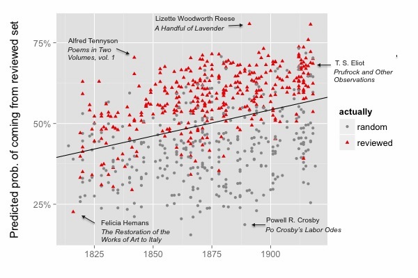
In the image above, each point is a volume of poetry, colored according to its actual social provenance. The y axis expresses a statistical model’s prediction about that provenance: How likely is it that this volume came from the “reviewed” sample, based only on the words in the volume?
As you can see, the model does a pretty decent job of sorting the two samples. It’s not right all the time, because of course a volume’s reception is determined by a lot of factors other than language (politics, the whims of reviewers, social networks). But the model is right 79.2% of the time, which is often enough to suggest that volumes reviewed in prominent venues had something in common. The sort of poetic language that got reviewed is distinguished from other poetic traditions not just toward the twentieth century, as we had expected, but throughout this period.
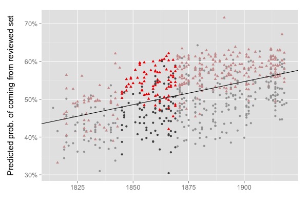
What’s even more puzzling is this: reviewed writers seem to have had the same thing in common throughout this century. The model is using essentially the same list of prestigious and banal words to separate Lord Byron from more obscure poets around 1819, and Christina Rossetti from more obscure poets around 1866, and T. S. Eliot from more obscure writers around 1917. That’s starting to sound like an oddly durable set of preferences. And actually, it’s even more durable than the image above suggests. A model trained on a quarter-century of the evidence can predict the other 75 years almost as accurately as a model trained on the whole century.
A model trained only on evidence from 1845-69 makes predictions about the other 75 years in the dataset.
So how is it even possible to characterize a whole century of poetic reception — based on fourteen different periodicals from both sides of the Atlantic — with a single set of aesthetic standards? Weren’t there supposed to be a couple of “poetic revolutions” in this century somewhere? W. B. Yeats certainly thought that one happened in the 1890s [2].
There’s another curious detail implied in the image above: why is the boundary between “reviewed” and “random” volumes drifting upward across the timeline? Technically, that’s an error. Volumes are not really “more likely to be reviewed” just because they were published later. But this is an error of an interesting kind. The model doesn’t know when these volumes were published: the dataset drifts upward because words that were more common in reviewed volumes across this period turn out to be more common in all volumes by the end of the period. If you divide the timeline into parts, the same pattern recurs in each part; and — to leak a detail from the next stage of this project — it also happens when we model fiction. That starts to suggest an interestingly general connection between synchronic judgment and diachronic change.
And there’s more. The detailed differences between reviewed and random poetry are interesting. In the article, we examine a haunting passage from Christina Rossetti; it turns out the model likes “haunting.” We also generalize about the theory of representativeness underpinning distant reading, and ask how our contemporary pedagogical canon looks when viewed by nineteenth-century aesthetic standards.
We’ve released our code and data on Github, and hope readers will find flaws in our reasoning so we can improve the project. But this draft has been bounced off a couple of audiences already; at this point it’s stable enough to be cited and criticized. So, after some reflection, we’ve closed comments on this post in order to encourage a more public sort of critique. If we’re overlooking something, please say so in a blog post. It’s an explicit premise of the project that “being reviewed at all indicates a sort of literary distinction — even if the review is negative.”
[1]: One influential thesis holds that this division crystallized “in the last decades of the 19th century and the first few years of the 20th.” Andreas Huyssen, After the Great Divide: Modernism, Mass Culture, Postmodernism (Bloomington: Indiana UP, 1986), viii.
[2]: W.B. Yeats dated the “revolt against Victorianism” and against “the poetical diction of everybody” to the 1890s. See discussion in Richard Fallis, “Yeats and the Reinterpretation of Victorian Poetry,” Victorian Poetry 14.2 (1976): 89-100.
If you haven’t read Ben’s blog post, I recommend exploring it now, because I’m going to skim lightly over some of the details of his method.
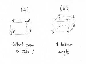
At its core, the technique is not complicated. It hinges on a transformation called principal component analysis (PCA), which allows researchers to map high-dimensional data onto a two-dimensional space, while keeping individual data points as far apart as possible. You can think of PCA as a technique that gives you a “good viewing angle” for flattening out a complex object. For instance, if you’ve got eight points at the corners of a cube, you could represent them as seen in (a), but (b) might be more legible because it spreads the points out more. It does that by squashing several different physical dimensions (length and breadth) into the x axis on the page.
Ben uses this technique to reveal the structural relationship between different parts of a plot. As I understand it, he divides television scripts into six segments of equal length, and trains a topic model on all the segments. If you produce, say, 100 topics, each segment of each show is now characterized as a point in 100-dimensional space, where each dimension measures the prominence of one particular topic.
He takes the first sixth of every show and averages them to produce a single point that represents the average topic distribution for the first-sixth of all shows. After doing that for all six segments, he has six data points that represent typical segments of narrative time. Then he uses PCA to find an abstract space where those points are well separated. When he does this, he gets an arc-like structure that tends to preserve the original narrative sequence of the segments (although the algorithm isn’t directly informed about sequence). In his most detailed visualization, he even takes this down to twelfths.
Benjamin Schmidt’s initial visualization of “plot arcs,” December 16, 2014.
But what does this mean?
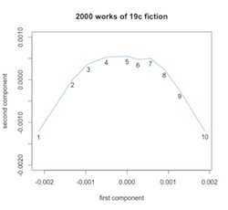
From the beginning, Ben has been pretty careful to stress that he sees the parabolic shape of this pattern as an artifact of PCA. (“I should emphasize that it’s hard to imagine any other shape coming out of the PCA algorithm with the inputs I put in.”) David Bamman confirms this, showing that PCA will turn many kinds of sequential data, even random walks, into an arc. The algorithm is also good at inferring sequence: if point 1 influences point 2, and point 2 influences point 3, etc., PCA will tend to preserve their sequential relationship in the projection. (It does this even if you take 1000 different random walks and add them up to produce a composite walk.) So if we believe that the topic distribution in each segment of each story is strongly related to the topic distributions on either side, we would expect PCA to organize the composite segments of all stories in a sequential arc.
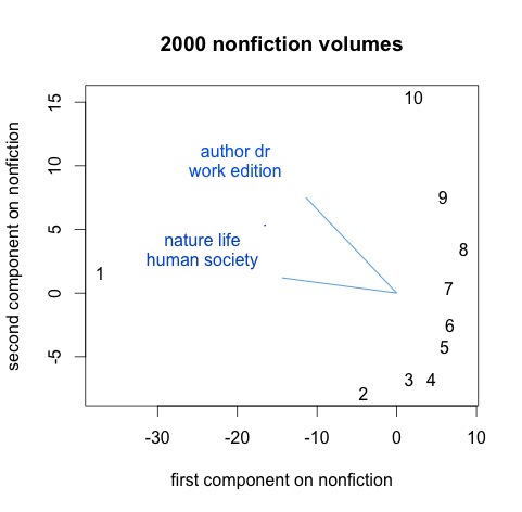
That’s sort of cool, but also suggests that the structure we’re seeing is not unique to “plots.” On the other hand, it’s worth noting that the technique does work better on fiction (and television scripts) than on nonfiction. Or, rather, it shows us something different when you apply it to nonfiction.
Here I’ve divided 2000 volumes of nineteenth-century nonfiction into ten parts, trained 200 topics on all 20,000 segments, and then created composite data points that represent the first “tenth,” second “tenth,” and so on, for all the volumes. PCA is still, somewhat remarkably, able to organize these points in the right sequence, but you have to squint a little to call this an arc. The graph is more clearly dominated by a contrast between introductions and body text. I’ve plotted two of the most important organizing topics as vectors; they include a lot of high-level abstractions and metadiscourse, whereas most of the topics in this nonfiction model are as specific as “birds eggs young wings” (and have a much smaller influence on this graph).
It’s important to note that I’m using the page-level metadata I recently described to select nonfiction here, which makes an effort to screen out paratext. (Otherwise we would probably be seeing topics like “table contents” and “index due date”!)
So where does this leave us? I think Lynn Cherny is right to say that with this technique, deviations from an arc are more significant than the arc itself. The slightly arc-like sequence on the right-hand side of the nonfiction graph isn’t telling us much about deep structures organizing nonfiction; it’s telling us mainly that there are continuities in text. But the “1” way over on the left-hand side is revealing a large structural fact: works of nonfiction have prefaces and introductions that can be very different from the rest of the text. Similarly, one of the most interesting aspects of Ben’s post involves the structural differences he finds toward the end between television genres (the difference between beginning and end seems more important for comedies, whereas science fiction is more organized by a contrast between central action and frame). Not a bad result for a historian to generate in his spare time.
Ten points that represent composite “tenths” of 1.981 works of fiction, topic-modeled and projected by PCA. Multivolume works have been joined.
Also, when I say differences are interesting, I don’t mean that the composite arc Ben saw by averaging all genres was meaningless. The fact that PCA will organize ten segments of 2000 novels into a parabola is not surprising. It would do that even with a random sequence. But in practice we’re not looking at random sequences, so PCA organizes points into a parabola by drawing on actual linguistic gradients that organize narrative time. As Ben has shown in a follow-up post, PCA is able to explain the patterns in television scripts better than it can explain random sequences.
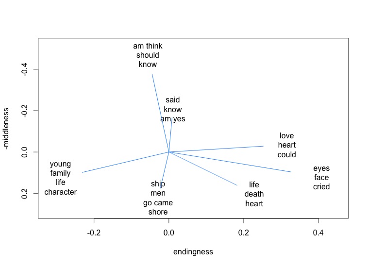
In other words, the differences we’re seeing between beginnings, middles, and ends are real differences. And it’s interesting to see what those differences are. The x and y axes in a PCA projection don’t have simple meanings, because we’ve squashed multiple dimensions into two. But we can understand the space a little better by mapping the influence exerted by different topics.
Vectors that play an especially strong role in organizing the PCA projection of 1,981 nineteenth-century novels.
In this visualization, for instance, topics associated with dialogue (“said am know yes”) tend to move a point up the y axis. They’re more common in the middle of a narrative.
It might also be interesting to compare the way narratives from different authors or genres project into this space.
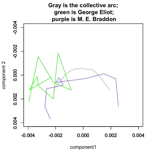
Each author here is represented by a composite set of ten segments of narrative time, produced by averaging her works. They are projected into a space defined by the average “tenths” of all works in the dataset.
Mary Elizabeth Braddon is a sensation novelist, and her works are strongly organized by a structure that resembles the majority of other novels in the nineteenth century (or is perhaps even more distinct than usual). A book like Lady Audley’s Secret begins with a stage-setting description of domestic space and family relationships. The middle of the book is characterized by dialogue. The tone of the diction becomes progressively more sentimental* until, in the conclusion, we back away from dialogue again to summary (but a summary that is very different from the introduction in tone).
By contrast, the novels of George Eliot are… um, perhaps it would be safest to say “not as well characterized by this model of narrative sequence.” You might be tempted to look at that tangle of lines and infer some kind of cyclic structure, but it would be a bit like reading tea leaves. I know George Eliot’s novels are interesting, but I doubt that squiggle tells me why. (It’s important to remember, for instance, that Eliot’s narrative time looks more orderly and arc-like when projected into a space defined by her own writing.)
Supervised and unsupervised models
In short, I think the method Ben has developed is interesting and worth further exploration, but I also think there are real interpretive challenges here. And the interpretive challenges are not general problems that would arise with any quantitative method: they’re specific to a quirk of this one, which is that it’s poised delicately between strategies of “supervised” and “unsupervised” modeling.
Actually, I’m not sure it’s technically accurate to call PCA a model at all; it’s almost a descriptive statistic (like the mean or standard deviation of a dataset). But the attraction of the technique is a bit like the attraction of unsupervised modeling: you turn it loose on the data and it spontaneously reveals patterns.
There’s nothing at all wrong with that, but the tricky thing here is that by focusing PCA on the temporal sequence within works, we actually give it a very strong bias toward a particular sort of pattern (a sequential arc). Which means we’re actually doing something that’s a bit more supervised than it might appear. It’s more like saying “if you assume narrative time is parabola-shaped, what would be the linguistic vectors organizing that space?”
All these approaches are interesting, and potentially valid; I just think it’s important to note that none of them are giving us an unsupervised model of plot. (Even unsupervised models do make assumptions, but I would say a topic model, for instance, is slightly more open-ended than an approach that implicitly maps sequences onto arcs.) There’s nothing wrong with assuming an arc, but there might be some advantage to doing it more explicitly. If I were going to use Ben’s insight to study plot in nineteenth-century novels, I would probably drop PCA and instead train two classifiers to recognize the “ends” and “middles” of narratives. When you do that, you get a result that is actually quite parallel to the one I got by using PCA.
The average probabilities two classifiers assigned to segments from different “tenths” of 1,981 novels. Five-fold crossvalidated, but I didn’t rule out the possibility that an author might appear in both the test set and the training set.
But with a predictive model like a classifier, I feel a little more confident in my ability to characterize the strength of the patterns I’m seeing. In this case, for instance, the classifier that recognizes ends was about 62% accurate out of sample. The classifier that recognizes middles was about 61% accurate, and since I counted six out of ten segments of each narrative as “the middle,” that’s not a lot better than random. [Later edit: This was a hasty first pass. Some simple normalization got the classifiers up to 67% and 64%. That signal is probably strong enough for people to do more interesting things with it.]
However, I want to be clear: I don’t think there’s anything wrong with using PCA for this, as long as we realize that it’s surprisingly good at inferring sequence from random walks in high-dimensional space. If plots are “arcs” (as critics have tended to assume), why not make use of that insight to analyze and visualize them? Ben’s post shows us one way to do that. Another thing I take away from this exploration is how amazing Twitter can be, because I couldn’t have fully understood what was going on here without contributions from a lot of different people.
* Re: “the tone of the diction becomes progressively more sentimental:” Matt Wilkens points out that the vectors that characterize endings here have a lot in common with the language that Sara Steger identified as characteristic of 19c sentimental fiction.
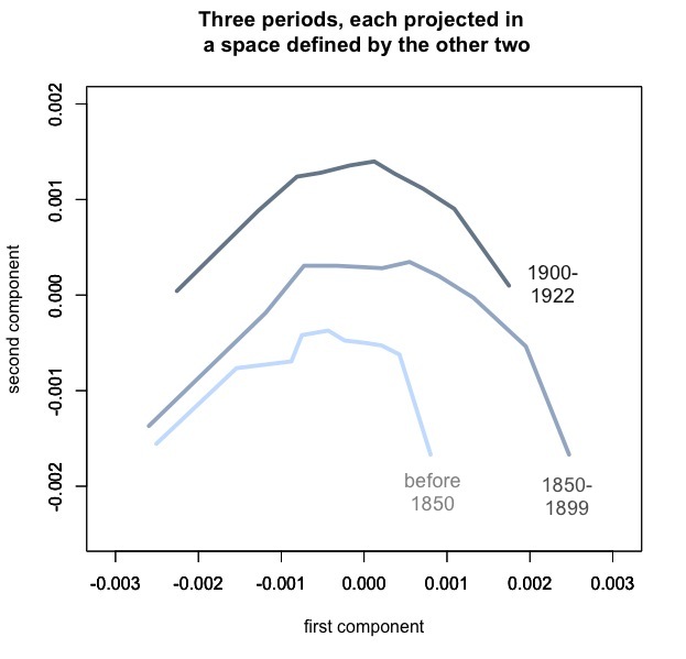
Postscript Jan 5: Have to admit I’ve found it hard to stop exploring this method. I ran it on a fiction dataset expanded to 4,000 works, and to 1922, and patterns started to become a little more legible. For instance, when I include more of her works, George Eliot no longer looks as idiosyncratic. It’s also kind of interesting to superimpose plot arcs for three different periods. Here I’ve borrowed Ben’s idea of using PCA so to speak “out-of-sample,” since each of these periods is actually projected into a different space (defined by the other two periods).
Generalized narrative arcs for 4,000 works of fiction from 1700 to 1922. In each case we’re plotting ten composite points representing the topic distributions for segments of narrative time, and time moves from left to right. The dataset does include reprints.
The fact that these arcs float upward may confirm something we already knew, which is that fiction tends to move away from “summary” and toward direct presentation of “scene” as historical time passes. But I think the stability of the pattern is also significant. As Ben has shown, there’s no guarantee that you’ll get an arc if you project a dataset into a PCA space defined by a different dataset. The congruence of these three arcs may not quite prove that plot *is* an arc, but it does suggest that linguistic signals of “beginnings,” “middles,” and “ends” remained broadly similar from the early nineteenth century through the early twentieth. If we wanted to confirm that, we could make more direct comparisons, but for exploratory visualization I see how PCA is useful here.
The relative sizes of different genres, represented as a percentage of pages in the English-language portion of HathiTrust. 854,476 volumes are covered. Nonfiction, front matter, and back matter aren't represented here. Results have been smoothed with a five-year moving average.
Although methods of analysis are more fun to discuss, the most challenging part of distant reading may still be locating the texts in the first place [1].
In principle, millions of books are available in digital libraries. But literary historians need collections organized by genre, and locating the fiction or poetry in a digital library is not as simple as it sounds. Older books don’t necessarily have genre information attached. (In HathiTrust, less than 40% of English-language fiction published before 1923 is tagged “fiction” in the appropriate MARC control field.)
Volume-level information wouldn’t be enough to guide machine reading in any case, because genres are mixed up inside volumes. For instance Hoyt Long, Richard So, and I recently published an article in Slate arguing (among other things) that references to specific amounts of money become steadily more common in fiction from 1825 to 1950.
Frequency of reference to “specific amounts” of money in 7,700 English-language works of fiction. Graphics here and throughout from Wickham, ggplot2 [2].
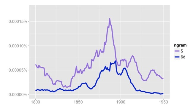
But Google’s “English Fiction” collection tells a very different story. The frequencies of many symbols that appear in prices (dollar signs, sixpence) skyrocket in the late nineteenth century, and then drop back by the early twentieth.
Frequencies of “$” and “6d” in Google’s “English Fiction” collection, 1800-1950.
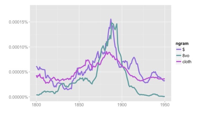
Frequencies of “$”, “8vo” (octavo) and “cloth” in Google’s “English Fiction” collection, 1800-1950.
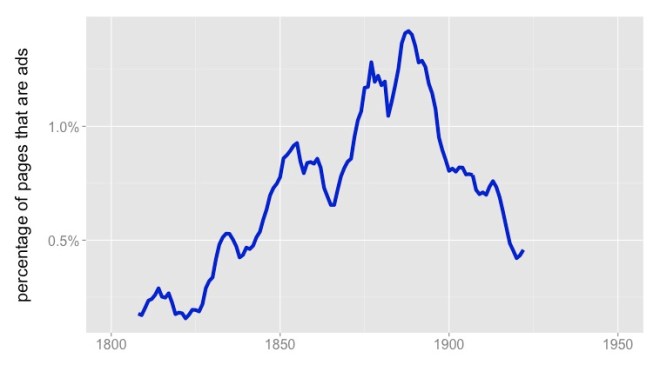
What we see in Google’s “Fiction” collection is something that happens in volumes of fiction, but not exactly in the genre of fiction — the rise and fall of publishers’ catalogs in the backs of books [3]. Individually, these two- or three-page lists of titles for sale may not look like significant noise, but because they often mention prices, and are distributed unevenly across the timeline, they add up to a significant potential pitfall for anyone interested in the role of money in fiction.
I don’t say this to criticize the team behind the Ngram Viewer. Genre wasn’t central to their goals; they provided a rough “fiction” collection merely as a cherry on top of a massively successful public-humanities project. My point is just that genres fail to line up with volume boundaries in ways that can really matter for the questions scholars want to pose. (In fact, fiction may be the genre that comes closest to lining up with volume boundaries: drama and poetry often appear mixed in The Collected Poems and Plays of So-and-So, With a Prose Life of the Author.)
You can solve this problem by selecting works manually, or by borrowing proprietary collections from a vendor. Those are both good, practical solutions, especially up to (say) 1900. But because they rely on received bibliographies, they may not entirely fulfill the promises we’ve been making about dredging the depths of “the great unread,” boldly going where no one has gone before, etc [4]. Over the past two years, with support from the ACLS and NEH, I’ve been trying to develop another alternative — a way of starting with a whole library, and dividing it by genre at the page level, using machine learning.
In researching the Slate article, we relied on that automatic mapping of genre to select pages of fiction from HathiTrust. It helped us avoid conflating advertisements with fiction, and I hope other scholars will also find that it reduces the labor involved in creating large, genre-specific collections. The point of this blog post is to announce the release of a first version of the map we used (covering 854,476 English-language books in HathiTrust 1700-1922).
We identify pages as paratext (front matter, back matter, ads), prose nonfiction, poetry (narrative and lyric are grouped together), drama (including verse drama), or prose fiction. The report discusses the rationale for these choices, but other choices would be possible.
“How accurate is this map?”
Since genres are social institutions, questions about accuracy are relative to human dissensus. Our pairs of human readers agreed about the five categories just mentioned for 94.5% of the pages they tagged [5]. Relying on two-out-of-three voting (among other things), we boiled those varying opinions down to a human consensus, and our model agreed with the consensus 93.6% of the time. So this map is nearly as accurate as we might expect crowdsourcing to be. But it covers 276 million pages. For full details, see the confusion matrices in the report. Also, note that we provide ways of adjusting the tradeoff between recall and precision to fit a researcher’s top priority — which could be catching everything that might belong in a genre, or filtering out everything that doesn’t belong. We provide filtered collections of drama, fiction, and poetry for scholars who want to work with datasets that are 97-98% precise.
The short answer: we can’t. I don’t expect the genre predictions in this dataset to be more than one resource among many. We’ve also designed this dataset to have a certain amount of flexibility. There are confidence metrics associated with each volume, and users can define their collection of, say, poetry more broadly or narrowly by adjusting the confidence thresholds for inclusion. So even this dataset is not really a single map.
“What about divisions below the page level?”
With the exception of divisions between running headers and body text, we don’t address them. There are certainly a wide range of divisions below the page level that can matter, but we didn’t feel there was much to be gained by trying to solve all those problems at the same time as page-level mapping. In many cases, divisions below the page level are logically a subsequent step.
“How would I actually use this map to find stuff?”
There are three different ways — see “How to use this data?” in the interim report. If you’re working with HathiTrust Research Center, you could use this data to define a workset in their portal. Alternatively, if your research question can be answered with word frequencies, you could download public page-level features from HTRC and align them with our genre predictions on your own machine to produce a dataset of word counts from “only pages that have a 97% probability of being prose fiction,” or what have you. (HTRC hasn’t released feature counts for all the volumes we mapped yet, but they’re about to.) You can also align our predictions directly with HathiTrust zip files, if you have those. The pagealigner module in the utilities subfolder of our Github repo is intended as a handy shortcut for people who use Python; it will work both with HT zip files and HTRC feature files, aligning them with our genre predictions and returning a list of pages zipped with genre codes.
Is this sort of collection really what I need for my project?
Maybe not. There are a lot of books in HathiTrust. But as I admitted in my last post, a medium-sized collection based on bibliographies may be a better starting point for most scholars. Library-based collections include things like reprints, works in translation, juvenile fiction, and so on, that could be viewed as giving a fuller picture of literary culture … or could be viewed as messy complicating factors. I don’t mean to advocate for a library-based approach; I’m just trying to expand the range of alternatives we have available.
“What if I want to find fiction in French books between 1900 and 1970?”
Although we’ve made our code available as a resource, we definitely don’t want to represent it as a “tool” that could simply be pointed at other collections to do the same kind of genre mapping. Much of the work involved in this process is domain-specific (for instance, you have to develop page-level training data in a particular language and period). So this is better characterized as a method than a tool, and the report is probably more important than the repo. I plan to continue expanding the English-language map into the twentieth century (algorithmic mapping of genre may in fact be especially necessary for distant reading behind the veil of copyright). But I don’t personally have plans to expand this map to other languages; I hope someone else will take up that task.
As a reward for reading this far, here’s a visualization of the relative sizes of genres across time, represented as a percentage of pages in the English-language portion of HathiTrust.
The relative sizes of different genres, represented as a percentage of pages in the English-language portion of HathiTrust. 854,476 volumes are covered. Nonfiction, front matter, and back matter aren’t represented here. Results have been smoothed with a five-year moving average. Click through to enlarge.
The blog post above often slips awkwardly into first-person plural, because I’m describing a project that involved a lot of people. Parts of the code involved were written by Michael L. Black and Boris Capitanu. The code also draws on machine learning libraries in Weka and Scikit-Learn [6, 7]. Shawn Ballard organized the process of gathering training data, assisted by Jonathan Cheng, Nicole Moore, Clara Mount, and Lea Potter. The project also depended on collaboration and conversation with a wide range of people at HathiTrust Digital Library, HathiTrust Research Center, and the University of Illinois Library, including but not limited to Loretta Auvil, Timothy Cole, Stephen Downie, Colleen Fallaw, Harriett Green, Myung-Ja Han, Jacob Jett, and Jeremy York. Jana Diesner and David Bamman offered useful advice about machine learning. Essential material support was provided by a Digital Humanities Start-Up Grant from the National Endowment for the Humanities and a Digital Innovation Fellowship from the American Council of Learned Societies. None of these people or agencies should be held responsible for mistakes.
References
[1] Perhaps it goes without saying, since the phrase has now lost its quotation marks, but “distant reading” is Franco Moretti, “Conjectures on World Literature,” New Left Review 1 (2000).
[2] Hadley Wickham, ggplot2: Elegant Graphics for Data Analysis.http: //had.co.nz/ggplot2/book. Springer New York, 2009.
[3] Having mapped advertisements in volumes of fiction, I’m pretty certain that they’re responsible for the spike in dollar signs in Google’s “English Fiction” collection. The collection I mapped overlaps heavily with Google Books, and the number of pages of ads in fiction volumes tracks very closely with the frequency of dollars signs, “8vo,” and so on.
Percentage of pages in mostly-fiction volumes that are ads. Based on a filtered collection of 102,349 mostly-fiction volumes selected from a larger group of 854,476 volumes 1700-1922. Five-year moving average.
[4] “The great unread” comes from Margaret Cohen, The Sentimental Education of the Novel (Princeton NJ: Princeton University Press, 1999), 23.
[5] See the interim report (subsection, “Evaluating Confusion Matrices”) for a fuller description; it gets complicated, because we actually assessed accuracy in terms of the number of words misclassified, although the classification was taking place at a page level.
[6] F. Pedregosa, G. Varoquaux, A. Gramfort, V. Michel, B. Thirion, O. Grisel, M. Blondel, P. Prettenhofer, R. Weiss, V. Dubourg, J. Vanderplas, A. Passos, D. Cournapeau, M. Brucher, M. Perrot, and E. Duchesnay. Scikit-learn: Machine learning in Python. Journal of Machine Learning Research, 12:2825–2830, 2011.
[7] Mark Hall, Eibe Frank, Geoffrey Holmes, Bernhard Pfahringer, Peter Reutemann, and Ian H. Witten. The WEKA data mining software: An update. SIGKDD Explorations, 11(1), 2009.
There are basically two different ways to build collections for distant reading. You can build up collections of specific genres, selecting volumes that you know belong to them. Or you can take an entire digital library as your base collection, and subdivide it by genre.
Most people do it the first way, and having just spent two years learning to do it the second way, I’d like to admit that they’re right. There’s a lot of overhead involved in mining a library. The problem becomes too big for your desktop; you have to schedule batch jobs; you have to learn to interpret MARC records. All this may be necessary eventually, but it’s not the ideal place to start.
But some of the problems I’ve encountered have been interesting. In particular, the problem of “dividing a library by genre” has made me realize that literary studies is constituted by exclusions that are a bit larger and more arbitrary than I used to think.
First of all, why is dividing by genre even a problem? Well, most machine-readable catalog records don’t say much about genre, and even if they did, a single volume usually contains multiple genres anyway. (Think introductions, indexes, collected poems and plays, etc.) With support from the ACLS and NEH, I’ve spent the last year wrestling with that problem, and in a couple of weeks I’m going to share an imperfect page-level map of genre for English-language books in HathiTrust 1700-1923.
But the bigger thing I want to report is that the ambiguity of genre may run deeper than most scholars who aren’t librarians currently imagine. To be sure, we know that subgenres like “detective fiction” are social institutions rather than natural forms. And in a vague way we also accept that broader categories like “fiction” and “poetry” are social constructs with blurry edges. We can all point to a few anomalies: prose poems, eighteenth-century journalistic fictions like The Spectator, and so on.
But somehow, in spite of knowing this for twenty years, I never grasped the full scale of the problem. For instance, I knew the boundary between fiction and nonfiction was blurry in the 18c, but I thought it had stabilized over time. By the time you got to the Victorians, surely, you could draw a circle around “fiction.” Exceptions would just prove the rule.
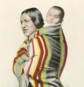
Selecting volumes one by one for genre-specific collections didn’t shake my confidence. But if you start with a whole library and try to winnow it down, you’re forced to consider a lot of things you would otherwise never look at. I’ve become convinced that the subset of genre-typical cases (should we call them cis-genred volumes?) is nowhere near as paradigmatic as literary scholars like to imagine. A substantial proportion of the books in a library don’t fit those models. This is both a photograph of a real, unnamed mother and baby, and a picture of a fictional character named Shinkah. Frontispiece to Shinkah, The Osage Indian (1916).
Consider the case of Shinkah, the Osage Indian, published in 1916 by S. M. Barrett. The preface to this volume informs us that it’s intended as a contribution to “the sociology of the Osage Indians.” But it’s set a hundred years in the past, and the central character Shinkah is entirely fictional (his name just means “child.”) On the other hand, the book is illustrated with photographs of real contemporary people, who stand for the characters in an ethnotypical way.
After wading though 872,000 volumes, I’m sorry to report that odd cases of this kind are more typical of nineteenth- and early twentieth-century fiction than my graduate-school training had led me to believe. There’s a smooth continuum for instance between Shinkah and Old Court Life in France (1873), by Frances Elliot. This book has a bibliography, and a historiographical preface, but otherwise reads like a historical novel, complete with invented dialogue. I’m not sure how to distinguish it from other historical novels with real historical personages as characters.
Literary critics know there’s a problem with historical fiction. We also know about the blurry boundary between fiction, journalism, and travel writing represented by the genre of the “sketch.” And anyone who remembers James Frey being kicked out of Oprah Winfrey’s definition of nonfiction knows that autobiographies can be problematic. And we know that didactic fiction blurs into philosophical dialogue. And anyone who studies children’s literature knows that the boundary between fiction and nonfiction gets especially blurry there. And probably some of us know about ethnographic novels like Shinkah. But I’m not sure many of us (except for librarians) have added it all up. When you’re sorting through an entire library you’re forced to see the scale of it: in the period 1700-1923, maybe 10% of the volumes that could be cataloged as fiction present puzzling boundary cases.
You run into a lot of these works even if you browse or select titles at random; that’s how I met Shinkah. But I’ve also been training probabilistic models of genre that report, among other things, how certain or uncertain they are about each page. These models are good at identifying clear cases of our received categories; I found that they agreed with my research assistants almost exactly as often as the research assistants agreed with each other (93-94% of the time, about broad categories like fiction/nonfiction). But you can also ask a model to sift through several thousand volumes looking for hard cases. When I did that I was taken aback to discover that about half the volumes it had most trouble with were things I also found impossible to classify. The model was most uncertain, for instance, about The Terrific Register (1825) — an almanac that mixes historical anecdote, urban legend, and outright fiction randomly from page to page. The second-most puzzling book was Madagascar, or Robert Drury’s Journal (1729), a book that offers itself as a travel journal by a real person, and was for a long time accepted as one, although scholars have more recently argued that it was written by Defoe.
Of course, a statistical model of fiction doesn’t care whether things “really happened”; it pays attention mostly to word frequency. Past-tense verbs of speech, personal names, and “the,” for instance, are disproportionately common in fiction. “Is” and “also” and “mr” (and a few hundred other words) are common in nonfiction. Human readers probably think about genre in a more abstract way. But it’s not particularly miraculous that a model using word frequencies should be confused by the same examples we find confusing. The model was trained, after all, on examples tagged by human beings; the whole point of doing that was to reproduce as much as possible the contours of the boundary that separates genres for us. The only thing that’s surprising is that trawling the model through a library turns up more books right in the middle of the boundary region than our habits of literary attention would have suggested.
A lot of discussions of distant reading have imagined it as a move from canonical to popular or obscure examples of a (known) genre. But reconsidering our definitions of the genres we’re looking for may be just as important. We may come to recognize that “the novel” and “the lyric poem” have always been islands floating in a sea of other texts, widely read but never genre-typical enough to be replicated on English syllabi.
In the long run, this may require us to balance two kinds of inclusiveness. We already know that digital libraries exclude a lot. Allen Riddell has nicely demonstrated just how much: he concludes that there are digital scans for only about 58% of the novels listed in bibliographies as having been published between 1800 and 1836.
One way to ensure inclusion might be to start with those bibliographies, which highlight books invisible in digital libraries. On the other hand, bibliographies also make certain things invisible. The Terrific Register (1825), for instance, is not in Garside’s bibliography of early-nineteenth-century fiction. Neither is The Wonder-Working Water Mill (1791), to mention another odd thing I bumped into. These aren’t oversights; Garside et. al. acknowledge that they’re excluding certain categories of fiction from their conception of the novel. But because we’re trained to think about novels, the scale of that exclusion may only become visible after you spend some time trawling a library catalog.
I don’t want to present this as an aporia that makes it impossible to know where to start. It’s not. Most people attempting distant reading are already starting in the right place — which is to build up medium-sized collections of familiar generic categories like “the novel.” The boundaries of those categories may be blurrier than we usually acknowledge. But there’s also such a thing as fretting excessively about the synchronic representativeness of your sample. A lot of the interesting questions in distant reading are actually trends that involve relative, diachronic differences in the collection. Subtle differences of synchronic coverage may more or less drop out of questions about change over time.
On the other hand, if I’m right that the gray areas between (for instance) fiction and nonfiction are bigger and more persistently blurry than literary scholarship usually mentions, that’s probably in the long run an issue we should consider! When I release a page-level map of genre in a couple of weeks, I’m going to try to provide some dials that allow researchers to make more explicit choices about degrees of inclusion or exclusion.
Predictive models that report probabilities give us a natural way to handle this, because they allow us to characterize every boundary as a gradient, and explicitly acknowledge our compromises (for instance, trade-offs between precision and recall). People who haven’t done much statistical modeling often imagine that numbers will give humanists spuriously clear definitions of fuzzy concepts. My experience has been the opposite: I think our received disciplinary practices often make categories seem self-evident and stable because they teach us to focus on easy cases. Attempting to model those categories explicitly, on a large scale, can force you to acknowledge the real instability of the boundaries involved.
References and acknowledgments
Training data for this project was produced by Shawn Ballard, Jonathan Cheng, Lea Potter, Nicole Moore and Clara Mount, as well as me. Michael L. Black and Boris Capitanu built a GUI that helped us tag volumes at the page level. Material support was provided by the National Endowment for the Humanities and the American Council of Learned Societies. Some information about results and methods is online as a paper and a poster, but much more will be forthcoming in the next month or so — along with a page-level map of broad genre categories and types of paratext.
The project would have been impossible without help from HathiTrust and HathiTrust Research Center. I’ve also been taught to read MARC records by librarians and information scientists including Tim Cole, M. J. Han, Colleen Fallaw, and Jacob Jett, any of whom could teach a course on “Cursed Metadata in Theory and Practice.”
I mention Garside’s bibliography of early nineteenth-century fiction. This is Garside, Peter, and Rainer Schöwerling. The English novel, 1770-1829 : a bibliographical survey of prose fiction published in the British Isles. Ed. Peter Garside, James Raven, and Rainer Schöwerling. 2 vols. Oxford: Oxford University Press, 2000.
The Institute of Electrical and Electronics Engineers is an odd venue for literary history, and our paper ends up touching so many disciplinary bases that it may be distracting.* So I thought I’d pull out four issues of interest to humanists and discuss them briefly here; I’m also taking the occasion to add a little information about gender that we uncovered too late to include in the paper itself.
1) The overall point about genre. Our title, “Mapping Mutable Genres in Structurally Complex Volumes,” may sound like the sort of impossible task heroines are assigned in fairy tales. But the paper argues that the blurry mutability of genres is actually a strong argument for a digital approach to their history. If we could start from some consensus list of categories, it would be easy to crowdsource the history of genre: we’d each take a list of definitions and fan out through the archive. But centuries of debate haven’t yet produced stable definitions of genre. In that context, the advantage of algorithmic mapping is that it can be comprehensive and provisional at the same time. If you change your mind about underlying categories, you can just choose a different set of training examples and hit “run” again. In fact we may never need to reach a consensus about definitions in order to have an interesting conversation about the macroscopic history of genre.
2) A workset of 32,209 volumes of English-language fiction. On the other hand, certain broad categories aren’t going to be terribly controversial. We can probably agree about volumes — and eventually specific page ranges — that contain (for instance) prose fiction and nonfiction, narrative and lyric poetry, and drama in verse, or prose, or some mixture of the two. (Not to mention interesting genres like “publishers’ ads at the back of the volume.”) As a first pass at this problem, we extract a workset of 32,209 volumes containing prose fiction from a collection of 469,200 eighteenth- and nineteenth-century volumes in HathiTrust Digital Library. The metadata for this workset is publicly available from Illinois’ institutional repository. More substantial page-level worksets will soon be produced and archived at HathiTrust Research Center.
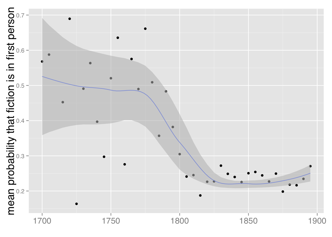
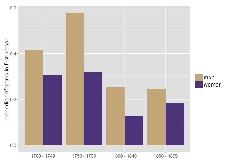
3) The declining prevalence of first-person narration. Once we’ve identified this fiction workset, we switch gears to consider point of view — frankly, because it’s a temptingly easy problem with clear literary significance. Though the fiction workset we’re using is defined more narrowly than it was last February, we confirm the result I glimpsed at that point, which is that the prevalence of first-person point of view declines significantly toward the end of the eighteenth century and then remains largely stable for the nineteenth.
Mean probability that fiction is written in first person, 1700-1899. Based on a corpus of 32,209 volumes of fiction extracted from HathiTrust Digital Library. Points are mean probabilities for five-year spans of time; a trend line with standard errors has been plotted with loess smoothing.
We can also confirm that result in a way I’m finding increasingly useful, which is to test it in a collection of a completely different sort. The HathiTrust collection includes reprints, which means that popular works have more weight in the collection than a novel printed only once. It also means that many volumes carry a date much later than their first date of publication. In some ways this gives a more accurate picture of print culture (an approximation to “what everyone read,” to borrow Scott Weingart’s phrase), but one could also argue for a different kind of representativeness, where each volume would be included only once, in a record dated to its first publication (an attempt to represent “what everyone wrote”).
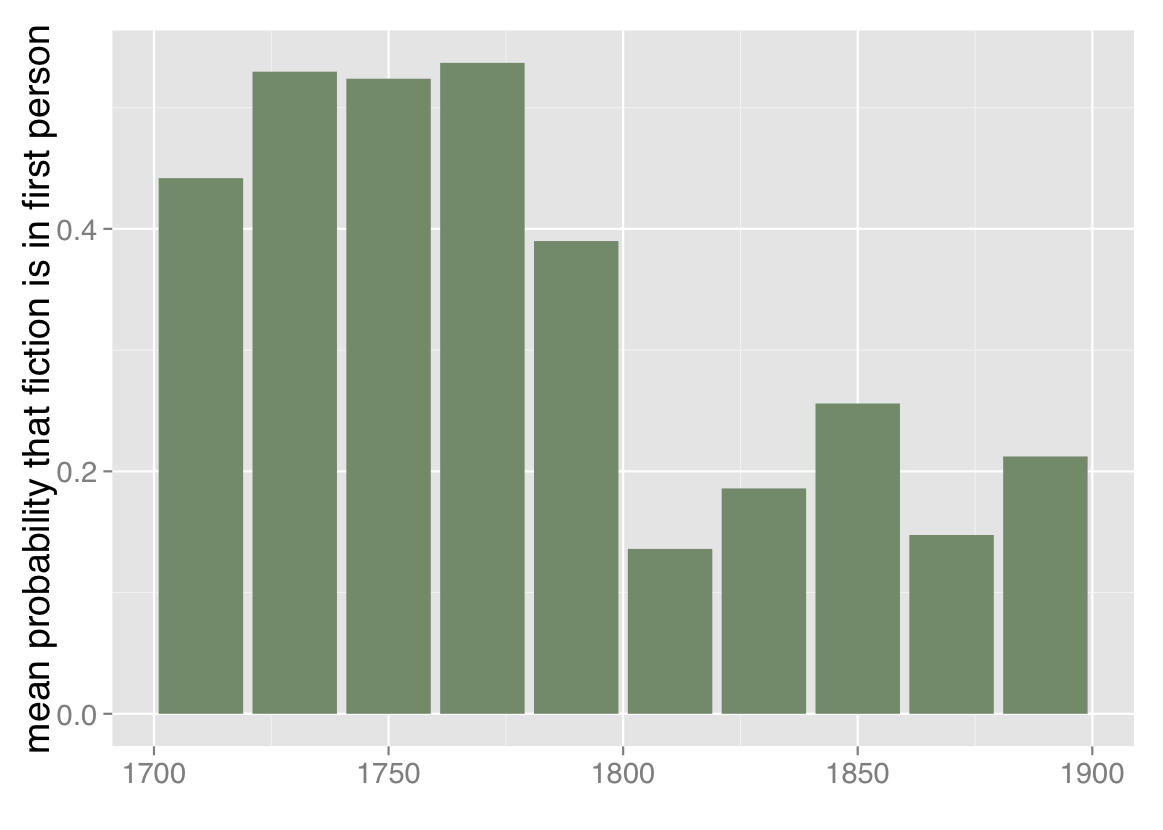
Mean probability that fiction is written in first person, 1700-1899. Based on a corpus of 774 volumes of fiction selected by multiple hands from multiple sources. Plotted in 20-year bins because n is smaller here. Works are weighted by the number of words they contain.
Fortunately, Jordan Sellers and I produced a collection like that a few years ago, and we can run the same point-of-view classifier on this very different set of 774 fiction volumes (metadata available), selected by multiple hands from multiple sources (including TCP-ECCO, the Brown Women Writers Project, and the Internet Archive). Doing that reveals broadly the same trend line we saw in the HathiTrust collection. No collection can be absolutely representative (for one thing, because we don’t agree on what we ought to be representing). But discovering parallel results in collections that were constructed very differently does give me some confidence that we’re looking at a real trend.
4. Gender and point of view. In the process of classifying works of fiction, we stumbled on interesting thematic patterns associated with point of view. Features associated with first-person perspective include first-person pronouns, obviously, but also number words and words associated with sea travel. Some of this association may be explained by the surprising persistence of a particular two-century-long genre, the Robinsonade. A castaway premise obviously encourages first-person narration, but the colonial impulse in the Robinsonade also seems to have encouraged acquisitive enumeration of the objects (goats, barrels, guns, slaves) its European narrators find on ostensibly deserted islands. Thus all the number words. (But this association of first-person perspective with colonial settings and acquisitive enumeration may well extend beyond the boundaries of the Robinsonade to other genres of adventure fiction.)
Third-person perspective, on the other hand, is durably associated with words for domestic relationships (husband, lover, marriage). We’re still trying to understand these associations; they could be consequences of a preference for third-person perspective in, say, courtship fiction. But third-person pronouns correlate particularly strongly with words for feminine roles (girl,daughter,woman) — which suggests that there might also be a more specifically gendered dimension to this question.
Since transmitting our paper to the IEEE I’ve had a chance to investigate this hypothesis in the smaller of the two collections we used for that paper — 774 works of fiction between 1700 and 1899: 521 by men, 249 by women, and four not characterized by gender. (Mike Black and Jordan Sellers recorded this gender data by hand.) In this collection, it does appear that male writers choose first-person perspective significantly more than women do. The gender gap persists across the whole timespan, although it might be fading toward the end of the nineteenth century.
Proportion of works of fiction by men and women in first person. Based on the same set of 774 volumes described above. (This figure counts strictly by the number of works rather than weighting works by the number of words they contain.)
Over the whole timespan, women use first person in roughly 23% of their works, and men use it in roughly 35% of their works.** That’s not a huge difference, but in relative terms it’s substantial. (Men are using first person 52% more than women). The Bayesian mafia have made me wary of p-values, but if you still care: a chi-squared test on the 2×2 contingency table of gender and point of view gives p < 0.001. (Attentive readers may already be wondering whether the decline of first person might be partly explained by an increase in the proportion of women writers. But actually, in this collection, works by women have a distribution that skews slightly earlier than that of works by men.)
These are very preliminary results. 774 volumes is a small set when you could test 32,209. At the recent HTRC Uncamp, Stacy Kowalczyk described a method for gender identification in the larger HathiTrust corpus, which we will be eager to borrow once it’s published. Also, the mere presence of an association between gender and point of view doesn’t answer any of the questions literary critics will really want to pose about this phenomenon — like, why is point of view associated with gender? Is this actually a direct consequence of gender, or is it an indirect consequence of some other variable like genre? Does this gendering of narrative perspective really fade toward the end of the nineteenth century? I don’t pretend to have answered any of those questions, all I’m doing here is flagging the existence of an interesting open question that will deserve further inquiry.
** We don’t actually represent point of view as a binary choice between first person or third person; the classifier reports probabilities as a continuous range between 0 and 1. But for purposes of this blog post I’ve simplified by dividing the works into two sets at the 0.5 mark. On this point, and for many other details of quantitative methodology, you’ll want to consult the paper itself.
Digital collections are vastly expanding literary scholars’ field of view: instead of describing a few hundred well-known novels, we can now test our claims against corpora that include tens of thousands of works. But because this expansion of scope has also raised expectations, the question of representativeness is often discussed as if it were a weakness rather than a strength of digital methods. How can we ever produce a corpus complete and balanced enough to represent print culture accurately?
I think the question is wrongly posed, and I’d like to suggest an alternate frame. As I see it, the advantage of digital methods is that we never need to decide on a single model of representation. We can and should keep enlarging digital collections, to make them as inclusive as possible. But no matter how large our collections become, the logic of representation itself will always remain open to debate. For instance, men published more books than women in the eighteenth century. Would a corpus be correctly balanced if it reproduced those disproportions? Or would a better model of representation try to capture the demographic reality that there were roughly as many women as men? There’s something to be said for both views.
To take another example, Scott Weingart has pointed out that there’s a basic tension in text mining between measuring “what was written” and “what was read.” A corpus that contains one record for every title, dated to its year of first publication, would tend to emphasize “what was written.” Measuring “what was read” is harder: a perfect solution would require sales figures, reviews, and other kinds of evidence. But, as a quick stab at the problem, we could certainly measure “what was printed,” by including one record for every volume in a consortium of libraries like HathiTrust. If we do that, a frequently-reprinted work like Robinson Crusoe will carry about a hundred times more weight than a novel printed only once.
We’ll never create a single collection that perfectly balances all these considerations. But fortunately, we don’t need to: there’s nothing to prevent us from framing our inquiry instead as a comparative exploration of many different corpora balanced in different ways.
For instance, if we’re troubled by the difference between “what was written” and “what was read,” we can simply create two different collections — one limited to first editions, the other including reprints and duplicate copies. Neither collection is going to be a perfect mirror of print culture. Counting the volumes of a novel preserved in libraries is not the same thing as counting the number of its readers. But comparing these collections should nevertheless tell us whether the issue of popularity makes much difference for a given research question.
I suspect in many cases we’ll find that it makes little difference. For instance, in tracing the development of literary language, I got interested in the relative prominence of words that entered English before and after the Norman Conquest — and more specifically, in how that ratio changed over time in different genres. My first approach to this problem was based on a collection of 4,275 volumes that were, for the most part, limited to first editions (773 of these were prose fiction).
But I recognized that other scholars would have questions about the representativeness of my sample. So I spent the last year wrestling with 470,000 volumes from HathiTrust; correcting their OCR and using classification algorithms to separate fiction from the rest of the collection. This produced a collection with a fundamentally different structure — where a popular work of fiction could be represented by dozens or scores of reprints scattered across the timeline. What difference did that make to the result? (click through to enlarge) The same question posed to two different collections. 773 hand-selected first editions on the left; on the right, 47,549 volumes, including many translations and reprints. Yearly ratios are plotted rather than individual works.
It made almost no difference. The scatterplots look different, of course, because the hand-selected collection (on the left) is relatively stable in size across the timespan, and has a consistent kind of noisiness, whereas the HathiTrust collection (on the right) gets so huge in the nineteenth century that noise almost disappears. But the trend lines are broadly comparable, although the collections were created in completely different ways and rely on incompatible theories of representation.
I don’t regret the year I spent getting a binocular perspective on this question. Although in this case changing the corpus made little difference to the result, I’m sure there are other questions where it will make a difference. And we’ll want to consider as many different models of representation as we can. I’ve been gathering metadata about gender, for instance, so that I can ask what difference gender makes to a given question; I’d also like to have metadata about the ethnicity and national origin of authors.
But the broader point I want to make here is that people pursuing digital research don’t need to agree on a theory of representation in order to cooperate.
If you’re designing a shared syllabus or co-editing an anthology, I suppose you do need to agree in advance about the kind of representativeness you’re aiming to produce. Space is limited; tradeoffs have to be made; you can only select one set of works.
But in digital research, there’s no reason why we should ever have to make up our minds about a model of representativeness, let alone reach consensus. The number of works we can select for discussion is not limited. So we don’t need to imagine that we’re seeking a correspondence between the reality of the past and any set of works. Instead, we can look at the past from many different angles and ask how it’s transformed by different perspectives. We can look at all the digitized volumes we have — and then at a subset of works that were widely reprinted — and then at another subset of works published in India — and then at three or four works selected as case studies for close reading. These different approaches will produce different pictures of the past, to be sure. But nothing compels us to make a final choice among them.
Of all our literary-historical narratives it is the history of criticism itself that seems most wedded to a stodgy history-of-ideas approach—narrating change through a succession of stars or contending schools. While scholars like John Guillory and Gerald Graff have produced subtler models of disciplinary history, we could still do more to complicate the narratives that organize our discipline’s understanding of itself.
A browsable network based on Underwood's model of PMLA. Click through, then mouse over or click on individual topics.The archive of scholarship is also, unlike many twentieth-century archives, digitized and available for “distant reading.” Much of what we need is available through JSTOR’s Data for Research API. So last summer it occurred to a group of us that topic modeling PMLA might provide a new perspective on the history of literary studies. Although Goldstone and Underwood are writing this post, the impetus for the project also came from Natalia Cecire, Brian Croxall, and Roger Whitson, who may do deeper dives into specific aspects of this archive in the near future.
Topic modeling is a technique that automatically identifies groups of words that tend to occur together in a large collection of documents. It was developed about a decade ago by David Blei among others. Underwood has a blog post explaining topic modeling, and you can find a practical introduction to the technique at the Programming Historian. Jonathan Goodwin has explained how it can be applied to the word-frequency data you get from JSTOR.
Obviously, PMLA is not an adequate synecdoche for literary studies. But, as a generalist journal with a long history, it makes a useful test case to assess the value of topic modeling for a history of the discipline.
Goldstone and Underwood each independently produced several different models of PMLA, using different software, stopword lists, and numbers of topics. Our results overlapped in places and diverged in places. But we’ve reached a shared sense that topic modeling can enrich the history of literary scholarship by revealing trends that are presently invisible.
What is a topic?
A “topic model” assigns every word in every document to one of a given number of topics. Every document is modeled as a mixture of topics in different proportions. A topic, in turn, is a distribution of words—a model of how likely given words are to co-occur in a document. The algorithm (called LDA) knows nothing “meta” about the articles (when they were published, say), and it knows nothing about the order of words in a given document.
This is a picture of 5940 articles from PMLA, showing the changing presence of each of 100 "topics" in PMLA over time. (Click through to enlarge; a longer list of topic keywords is here.) For example, the most probable words in the topic arbitrarily numbered 59 in the model visualized above are, in descending order:
che gli piu nel lo suo sua sono io delle perche questo quando ogni mio quella loro cosi dei
This is not a “topic” in the sense of a theme or a rhetorical convention. What these words have in common is simply that they’re basic Italian words, which appear together whenever an extended Italian text occurs. And this is the point: a “topic” is neither more nor less than a pattern of co-occurring words.
Nonetheless, a topic like topic 59 does tell us about the history of PMLA. The articles where this topic achieved its highest proportion were:
Antonio Illiano, “Momenti e problemi di critica pirandelliana: L’umorismo, Pirandello e Croce, Pirandello e Tilgher,” PMLA 83 no. 1 (1968): pp. 135-143
Domenico Vittorini, “I Dialogi ad Petrum Histrum di Leonardo Bruni Aretino (Per la Storia del Gusto Nell’Italia del Secolo XV),” PMLA 55 no. 3 (1940): pp. 714-720
Vincent Luciani, “Il Guicciardini E La Spagna,” PMLA 56 no. 4 (1941): pp. 992-1006
And here’s a plot of the changing proportions of this topic over time, showing moving 1-year and 5-year averages:
We see something about PMLA that is worth remembering for the history of criticism, namely, that it has embedded Italian less and less frequently in its language since midcentury. (The model shows that the same thing is true of French and German.)
What can topics tell us about the history of theory?
Of course a topic can also be a subject category—modeling PMLA, we have found topics that are primarily “about Beowulf” or “about music.” Or a topic can be a group of words that tend to co-occur because they’re associated with a particular critical approach.
Here, for instance, we have a topic from Underwood’s 150-topic model associated with discussions of pattern and structure in literature. We can characterize it by listing words that occur more commonly in the topic than elsewhere, or by graphing the frequency of the topic over time, or by listing a few articles where it’s especially salient.
At first glance this topic might seem to fit neatly into a familiar story about critical history. We know that there was a mid-twentieth-century critical movement called “structuralism,” and the prominence of “structure” here might suggest that we’re looking at the rise and fall of that movement. In part, perhaps, we are. But the articles where this topic is most prominent are not specifically “structuralist.” In the top four articles, Ferdinand de Saussure, Claude Lévi-Strauss, and Northrop Frye are nowhere in evidence. Instead these articles appeal to general notions of symmetry, or connect literary patterns to Neoplatonism and Renaissance numerology.
By forcing us to attend to concrete linguistic practice, topic modeling gives us a chance to bracket our received assumptions about the connections between concepts. While there is a distinct mid-century vogue for structure, it does not seem strongly associated with the concepts that are supposed to have motivated it (myth, kinship, language, archetype). And it begins in the 1940s, a decade or more before “structuralism” is supposed to have become widespread in literary studies. We might be tempted to characterize the earlier part of this trend as “New Critical interest in formal unity” and the latter part of it as “structuralism.” But the dividing line between those rationales for emphasizing pattern is not evident in critical vocabulary (at least not at this scale of analysis).
This evidence doesn’t necessarily disprove theses about the history of structuralism. Topic modeling might not reveal varying “rationales” for using a word even if those rationales did vary. The strictly linguistic character of this technique is a limitation as well as a strength: it’s not designed to reveal motivation or conflict. But since our histories of criticism are already very intellectual and agonistic, foregrounding the conscious beliefs of contending critical “schools,” topic modeling may offer a useful corrective. This technique can reveal shifts of emphasis that are more gradual and less conscious than the ones we tend to celebrate.
It may even reveal shifts of emphasis of which we were entirely unaware. “Structure” is a familiar critical theme, but what are we to make of this?
A fuller list of terms included in this topic would include “character”, “fact,” “choice,” “effect,” and “conflict.” Reading some of the articles where the topic is prominent, it appears that in this topic “point” is rarely the sort of point one makes in an argument. Instead it’s a moment in a literary work (e.g., “at the point where the rain occurs,” in Robert apRoberts 379). Apparently, critics in the 1960s developed a habit of describing literature in terms of problems, questions, and significant moments of action or choice; the habit intensified through the early 1980s and then declined. This habit may not have a name; it may not line up neatly with any recognizable school of thought. But it’s a fact about critical history worth knowing.
Note that this concern with problem-situations is embodied in common words like “way” and “cannot” as well as more legible, abstract terms. Since common words are often difficult to interpret, it can be tempting to exclude them from the modeling process. It’s true that a word like “the” isn’t likely to reveal much. But subtle, interesting rhetorical habits can be encoded in common words. (E.g. “itself” is especially common in late-20c theoretical topics.)
We don’t imagine that this brief blog post has significantly contributed to the history of criticism. But we do want to suggest that topic modeling could be a useful resource for that project. It has the potential to reveal shifts in critical vocabulary that aren’t well described, and that don’t fit our received assumptions about the history of the discipline.
Why browse topics as a network?
The fact that a word is prominent in topic A doesn’t prevent it from also being prominent in topic B. So certain generalizations we might make about an individual topic (for instance, that Italian words decline in frequency after midcentury) will be true only if there’s not some other “Italian” topic out there, picking up where the first one left off.
For that reason, interpreters really need to survey a topic model as a whole, instead of considering single topics in isolation. But how can you browse a whole topic model? We’ve chosen relatively small numbers of topics, but it would not be unreasonable to divide literary scholarship into, say, 500 topics. Information overload becomes a problem.
A browsable image map of 150 topics from PMLA. After you click through you can mouseover (or click) individual topics for more information.We’ve found network graphs useful here. Click on the image of the network on the right to browse Underwood’s 150-topic model. The size of each node (roughly) indicates the number of words in the topic; color indicates the average date of words. (Blue topics are older; yellow topics are more recent.) Topics are linked to each other if they tend to appear in the same articles. Topics have been labeled with their most salient word—unless that word was already taken for another topic, or seemed misleading. Mousing over a topic reveals a list of words associated with it; with most topics it’s also possible to click through for more information.
The structure of the network makes a loose kind of sense. Topics in French and German form separate networks floating free of the main English structure. Recent topics tend to cluster at the bottom of the page. And at the bottom, historical and pedagogical topics tend to be on the left, while formal, phenomenological, and aesthetic categories tend to be on the right.
But while it’s a little eerie to see patterns like this emerge automatically, we don’t advise readers to take the network structure too seriously. A topic model isn’t a network, and mapping one onto a network can be misleading. For instance, topics that are physically distant from each other in this visualization are not necessarily unrelated. Connections below a certain threshold go unrepresented.
Goldstone’s 100-topic model of PMLA; click through to enlarge.Moreover, as you can see by comparing illustrations in this post, a little fiddling with dials can turn the same data into networks with rather different shapes. It’s probably best to view network visualization as a convenience. It may help readers browse a model by loosely organizing topics—but there can be other equally valid ways to organize the same material.
How did our models differ?
The two models we’ve examined so far in this post differ in several ways at once. They’re based on different spans of PMLA‘s print run (1890–1999 and 1924–2006). They were produced with different software. Perhaps most importantly, we chose different numbers of topics (100 and 150).
But the models we’re presenting are only samples. Goldstone and Underwood each produced several models of PMLA, changing one variable at a time, and we have made some closer apples-to-apples comparisons.
Broadly, the conclusion we’ve reached is that there’s both a great deal of fluidity and a great deal of consistency in this process. The algorithm has to estimate parameters that are impossible to calculate exactly. So the results you get will be slightly different every time. If you run the algorithm on the same corpus with the same number of topics, the changes tend to be fairly minor. But if you change the number of topics, you can get results that look substantially different.
On the other hand, to say that two models “look substantially different” isn’t to say that they’re incompatible. A jigsaw puzzle cut into 100 pieces looks different from one with 150 pieces. If you examine them piece by piece, no two pieces are the same—but once you put them together you’re looking at the same picture. In practice, there was a lot of overlap between our models; on the older end of the spectrum you often see a topic like “evidence fact,” while the newer end includes topics that foreground narrative, rhetoric, and gender. Some of the more surprising details turned out to be consistent as well. For instance, you might expect the topic “literary literature” to skew toward the older end of the print run. But in fact this is a relatively recent topic in both of our models, associated with discussion of canonicity. (Perhaps the owl of Minerva flies only at dusk?)
Contrasting models: a short example
While some topics look roughly the same in all of our models, it’s not always possible to identify close correlates of that sort. As you vary the overall number of topics, some topics seem to simply disappear. Where do they go? For example, there is no exact counterpart in Goldstone’s model to that “structure” topic in Underwood’s model. Does that mean it is a figment? Underwood isolated the following article as the most prominent exemplar:
Robert E. Burkhart, The Structure of Wuthering Heights, Letter to the Editor, PMLA 87 no. 1 (1972): 104–5. (Incidentally, jstor has miscategorized this as a “full-length article.”)
Goldstone’s model puts more than half of Burkhart’s comment in three topics:
0.24 topic 38 time experience reality work sense form present point world human process structure concept individual reader meaning order real relationship
0.13 topic 46 novels fiction poe gothic cooper characters richardson romance narrator story novelist reader plot novelists character reade hero heroine drf
0.12 topic 13 point reader question interpretation meaning make reading view sense argument words word problem makes evidence read clear text readers
The other prominent documents in Underwood’s 109 are connected to similar topics in Goldstone’s model. The keywords for Goldstone’s topic 38, the top topic here, immediately suggest an affinity with Underwood’s topic 109. Now compare the time course of Goldstone’s 38 with Underwood’s 109 (the latter is above):
It is reasonable to infer that some portion of the words in Underwood’s “structure” topic are absorbed in Goldstone’s “time experience” topic. But “time experience reality work sense” looks less like vocabulary for describing form (although “form” and “structure” are included in it, further down the list; cf. the top words for all 100 topics), and more like vocabulary for talking about experience in generalized ways—as is also suggested by the titles of some articles in which that topic is substantially present:
“The Vanishing Subject: Empirical Psychology and the Modern Novel”
“Metacommentary”
“Toward a Modern Humanism”
“Wordsworth’s Inscrutable Workmanship and the Emblems of Reality”
This version of the topic is no less “right” or “wrong” than the one in Underwood’s model. They both reveal the same underlying evidence of word use, segmented in different but overlapping ways. Instead of focusing our vision on affinities between “form” and “structure”, Goldstone’s 100-topic model shows a broader connection between the critical vocabulary of form and structure and the keywords of “humanistic” reflection on experience.
The most striking contrast to these postwar themes is provided by a topic which dominates in the prewar period, then gives way before “time experience” takes hold. Here are box plots by ten-year intervals of the proportions of another topic, Goldstone’s topic 40, in PMLA articles:
Underwood’s model shows a similar cluster of topics centering on questions of evidence and textual documentation, which similarly decrease in frequency. The language of PMLA has shown a consistently declining interest in “evidence found fact” in the era of the postwar research university.
So any given topic model of a corpus is not definitive. Each variation in the modeling parameters can produce a new model. But although topic models vary, models of the same corpus remain fundamentally consistent with each other.
Using LDA as evidence
It’s true that a “topic model” is simply a model of how often words occur together in a corpus. But information of that kind has a deeper significance than we might at first assume. A topic model doesn’t just show you what people are writing about (a list of “topics” in our ordinary sense of the word). It can also show you how they’re writing. And that “how” seems to us a strong clue to social affinities—perhaps especially for scholars, who often identify with a methodology or critical vocabulary. To put this another way, topic modeling can identify discourses as well as subject categories and embedded languages. Naturally we also need other kinds of evidence to produce a history of the discipline, including social and institutional evidence that may not be fully manifest in discourse. But the evidence of topic modeling should be taken seriously.
As you change the number of topics (and other parameters), models provide different pictures of the same underlying collection. But this doesn’t mean that topic modeling is an indeterminate process, unreliable as evidence. All of those pictures will be valid. They are taken (so to speak) at different distances, and with different levels of granularity. But they’re all pictures of the same evidence and are by definition compatible. Different models may support different interpretations of the evidence, but not interpretations that absolutely conflict. Instead the multiplicity of models presents us with a familiar choice between “lumping” or “splitting” cultural phenomena—a choice where we have long known that multiple levels of analysis can coexist. This multiplicity of perspective should be understood as a strength rather than a limitation of the technique; it is part of the reason why an analysis using topic modeling can afford a richly detailed picture of an archive like PMLA.
Appendix: How did we actually do this?
The PMLA data obtained from JSTOR was independently processed by Goldstone and Underwood for their different LDA tools. This created some quantitative subtleties that we’ve saved for this appendix to keep this post accessible to a broad audience. If you read closely, you’ll notice that we sometimes talk about the “probability” of a term in a topic, and sometimes about its “salience.” Goldstone used MALLET for topic modeling, whereas Underwood used his own Java implementation of LDA. As a result, we also used slightly different formulas for ranking words within a topic. MALLET reports the raw probability of terms in each topic, whereas Underwood’s code uses a slightly more complex formula for term salience drawn from Blei & Lafferty (2009). In practice, this did not make a huge difference.
MALLET also has a “hyperparameter optimization” option which Goldstone’s 100-topic model above made use of. Before you run screaming, “hyperparameters” are just dials that control how much fuzziness is allowed in a topic’s distribution across words (beta) or across documents (alpha). Allowing alpha to vary allows greater differentiation between the sizes of large topics (often with common words), and smaller (often more specialized) topics. (See “Why Priors Matter,” Wallach, Mimno, and McCallum, 2009.) In any event, Goldstone’s 100-topic model used hyperparameter optimization; Underwood’s 150-topic model did not. A comparison with several other models suggests that the difference between symmetric and asymmetric (optimized) alpha parameters explains much of the difference between their structures when visualized as networks.
Goldstone’s processing scripts are online in a github repository. The same repository includes R code for making the plots from Goldstone’s model. Goldstone would also like to thank Bob Gerdes of Rutgers’s Office of Instructional and Research Technology for support for running mallet on the university’s apps.rutgers.edu server, Ben Schmidt for helpful comments at a THATCamp Theory session, and Jon Goodwin for discussion and his excellent blog posts on topic-modeling jstor data.