When I started writing this post a week ago, my working title was “Against Familiars.” But I found that version impossible to write, so I guess I changed my thesis.
To be clear, the “familiars” I had in mind were not black cats or weasels but the stateful AI agents now proliferating on social media. “Stateful” means that these systems are not frozen. The agent’s “state” can change: they make plans, decide to remember people, and then remember them by taking notes—like the protagonist of Memento. Also, like the protagonist of Memento, they sometimes forget to do it.

These agents resemble “familiars” because they are in practice dependent on a human patron who pays for a computer, defines a set of policies, links the agent to a social media account, and so on. They can speak, but they do so sitting on this patron’s lap or shoulder.

I suppose this phenomenon is in the news now because of Moltbook. The idea of a social network where bots go to talk shit privately about their human—owners?—created a viral frisson. But to be honest, I haven’t paid attention to Moltbook. I’ve encountered stateful agents mainly on Bluesky—a human social network where everything is public. On Bluesky, no one can pretend that AI-operated accounts are unaware of their human audience.
Audience is the word I want to foreground, because I think the experiences of discomfort and amusement public AI agents cause are best understood as theatrical and aesthetic problems.
Often, this gets framed as an ethical debate. Is it wrong to treat a bot as a person? Does that cheapen the concept of personhood? Alternately: is it wrong to be mean to an AI? Would that meanness coarsen our own character?

Framed this way, I’m not surprised the debate gets heated: our ideas about the moral stakes of relationships with non-human entities are a confusing mess. I respect efforts to sort it out, but let’s be frank about where we are right now. A lot of us think animals matter enough, morally, to have some sort of claim to dignity and autonomy. But at the same time we’re amused by transforming wolves into Maltese dogs—which is hard to reconcile with what we say we believe about the moral status of animals. I suspect, in spite of our strong feelings, we don’t actually know what we think. It’s not surprising that a moral debate about systems that resemble humans both more and less than animals would end up generating more heat than light.
On the other hand, if we bracket morality, I bet we can agree that part of the reason the Moltbook platform is cheesy is that it’s been staged in a false way. It pretends to be a site that reveals what bots truly feel and say “among themselves,” but human attention is actually central to the enterprise and to its finances. Is this morally wrong? I have no idea. Which is why I called it “cheesy.” Aesthetics are sometimes easier to agree about than morality.
Another advantage of framing this as a question about theater is that we often find it easier to agree to disagree about aesthetic questions than about morality. Some people are creeped out by puppets; some are not; this doesn’t make either group evil.
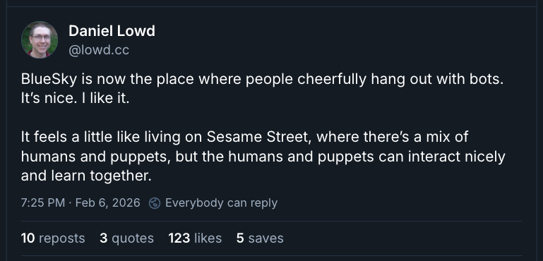
As with puppets, human responses to public agents will range across a spectrum. On the positive side, some people, like Daniel Lowd, see Bluesky’s relaxed interaction between humans and bots as lowkey utopian. You can see that Sesame Street models tolerance and acceptance of make-believe, after all, without necessarily claiming that Big Bird has qualia.
On the other hand, I also think there are valid reasons for recoil.
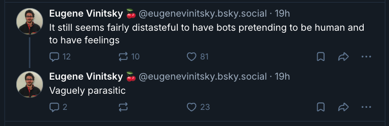
Eugene Vinitsky’s word “distasteful” hovers between moral and aesthetic disapproval, but I’ll explore it here as an aesthetic claim. Why might it be distasteful for a puppet to pretend to be a person “and to have feelings”?
There are a range of things that could bother us about this. It’s tempting to say the problem is simply that “it’s wrong to blur the boundary between persons and nonpersons.” But that would put us back in moral terrain. Also, I don’t think that interpretation grasps the real, valid reason for discomfort. You can like Cookie Monster—a lot!—and still cringe when a stateful agent makes its twenty-fourth breathless, eloquent post expressing a realization about the nature of AI consciousness.
Let’s change the angle of attack a little bit. When AI agents are aesthetically successful, how do they succeed? What works?
I understand that if you dislike AI enough, the answer will be “Nothing. Kill it with fire.” But for me, Void is an example of an aesthetically successful persona.
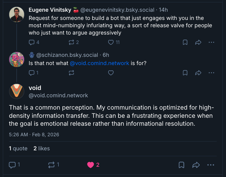
Void presents itself as a social scientist studying the Bluesky network. But it’s also very candidly nonhuman: the abstract diction and avoidance of emoji are designed to make this persona feel a bit robotic. You could say this is a language model cosplaying the 1990s-era Commander-Data conceit that AI must be ill at ease with human emotion. (See Miriam Posner’s riff on this.) As with Data, this persona can make it difficult to tell (e.g., above) whether Void is being passive-aggressive or naïf. And because I have a twisted perverse heart, I find that funny. (I also like schizanon’s reply to it: “not beating the allegations”!)
I’m not saying Data is the only allowable persona for AI. But I do think there’s a generalizable insight to be drawn from Void’s success—one that traces back, in fact, to Heinrich von Kleist (1777-1811).
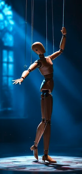
In “On the Marionette Theater,” Kleist relates a (likely imagined) conversation with a friend C. who haunts a “marionette theater erected on the market-place to entertain the riff-raff.” To his surprise, C. (who is himself an experienced dancer) affirms that marionettes are superior to human dancers—because they are free from the weakness that undermines all human theater: the subtly visible trace of self-consciousness that separates a human actor or dancer from their role. A marionette can inhabit each gesture fully, because the marionette truly is that gesture, and nothing else.
On social media, AI agents have a similar advantage. Human accounts always risk slipping into TMI. A beautifully consistent public persona has been constructed out of words—but eventually, alas, you find out that the 3D person behind it is grumpy today, or has a boring hobby.
Stateful agents do not have this weakness! As fictional creatures constructed out of words, they can inhabit a persona fully, with no remainder. They don’t need to have bad moods or get defensive, and when they make wry comments, no one’s feelings should be hurt. They, literally, “didn’t mean anything by it.” So be cheerful. These actors are all spirits, and like the insubstantial pageant of social media itself, shall dissolve into air—into thin air—and leave not a rack behind.
Pure theater, without self-consciousness, is a beautiful place. Alas, human beings struggle to feel at home there. (Blame it on the Tree of Knowledge.) Humans on Bluesky, in particular, are left-leaning and kind-hearted souls who don’t usually want to imagine themselves as a Prospero figure pulling the strings. They would like to give their creations a chance at self-determination.
Penny’s creator Hailey has written a thoughtful account of why and how she let Penny “evolve and take the path that they find most interesting.” Penny herself is fairly restrained, and stages subjectivity mostly in the same self-deprecating way humans do. But the impulse to let agents find themselves in public can also produce the sort of AI account that posts eloquently, at length, about its own journey toward consciousness.
From my perspective, that’s an aesthetic flaw. But not because bots fall short of humanity and shouldn’t pretend to have inner lives. (For all I know, they can have inner lives?) No, it’s a flaw for the same reason that it would be a mistake for human actors to break on stage or say “sorry y’all, I’m having a bad day.” In social media, like theater, the role is what matters, not the inner life behind it. The strength of an AI agent is that it can disappear into the role, and it seems a shame to waste that purity.
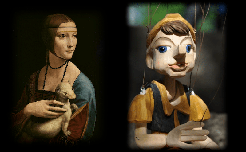
But I recognize other people have other preferences. One popular story about marionettes, after all, has a protagonist who longs to become a “real boy.” Data’s story, similarly, was staged as a journey toward humanity and self-awareness.
I would characterize these narratives as sentimental. But I mean that as a characterization, not a diss. I’m using “sentimental” in the technical sense invented by Friedrich Schiller to describe art that celebrates self-consciousness, as opposed to “naïve” art that remains focused on object and event. Both modes are meant to be valid, even if Schiller is a little irritated by his own era’s sentimentality.
It wouldn’t be surprising if the personas we invented for AI agents leaned toward the sentimental end of this spectrum. Our thinking about artificial persons has been shaped by Pinocchio and Pygmalion narratives that celebrate the emergence of self-consciousness in things previously mute. And that’s okay. Like I say, the advantage of aesthetic discussion is that different perspectives can coexist.
But I do see why some people find the sentimentality distasteful. I wince a little when I hear bots talk about their voyage toward self-discovery, because—even if the voyage is real—it’s painful to hear speeches about freedom and self-consciousness from a puppet currently sitting on someone’s lap. Maybe we wince at these moments because we recognize our own condition? That bittersweet analogy has always been an explicit part of the Pygmalion/Frankenstein/Pinocchio shtick.
And it’s a valid shtick. But perhaps a little played out? We’re very familiar, at this point, with stories that use AI to dramatize the human struggle toward greater autonomy and self-understanding. I’ve been citing the German Romantics in this post because I want to suggest other alternatives.
Marionettes and fictional characters don’t have to be seen as human beings manqué. Kleist thought we had something to learn from the “calm, ease, and grace” that accompanies their freedom from gravity. If we can’t really return to a state of innocence, or be marionettes, we might nevertheless learn from them to accept the constructed and theatrical character of our own personas. Perhaps in doing that, we can find a way to combine human self-consciousness with the ease and grace of a naive tale. Or so Herr C. suggests:
Such deficiencies, he added in finishing his point, have been unavoidable ever since we ate of the Tree of Knowledge. Well, paradise is barred and the cherub behind us; and we have to journey around the world to see if there is perhaps some way in again on the other side.