November 2011 – The Stone and the Shell

Exploring the relationship between topics and trends.

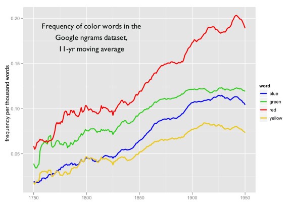
I’ve been talking about correlation since I started this blog. Actually, that was the reason why I did start it: I think literary scholars can get a huge amount of heuristic leverage out of the fact that thematically and socially-related words tend to rise and fall together. It’s a simple observation, and one that stares you in the face as soon as you start to graph word frequencies on the time axis.¹ But it happens to be useful for literary historians, because it tends to uncover topics that also pose periodizable kinds of puzzles. Sometimes the puzzle takes the form of a topic we intuitively recognize (say, the concept of “color”) that increases or decreases in prominence for reasons that remain to be explained:

At other times, the connection between elements of the topic is not immediately intuitive, but the terms are related closely enough that their correlation suggests a pattern worthy of further exploration. The relationship between terms may be broadly historical:

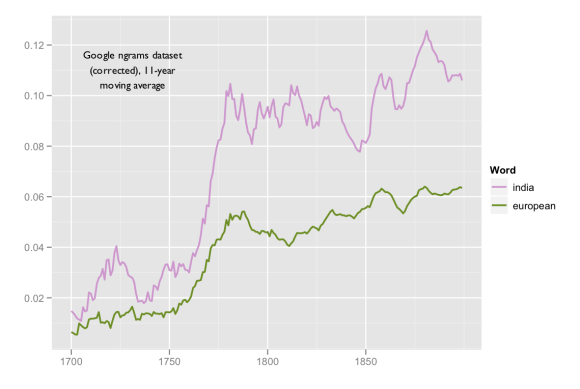
Or it may involve a pattern of expression that characterizes a periodizable style:

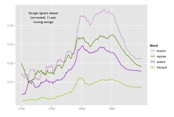
Of course, as the semantic relationship between terms becomes less intuitively obvious, scholars are going to wonder whether they’re looking at a real connection or merely an accidental correlation. “Ardent” and “tranquil” seem like opposites; can they really be related as elements of a single discourse? And what’s the relationship to “bosom,” anyway?

Ultimately, questions like this have to be addressed on a case-by-case basis; the significance of the lead has to be fleshed out both with further analysis, and with close reading.

But scholars who are wondering about the heuristic value of correlation may be reassured to know that this sort of lead does generally tend to pan out. Words that correlate with each other across the time axis do in practice tend to appear in the same kinds of volumes. For instance, if you randomly select pairs of words from the top 10,000 words in the Google English ngrams dataset 1700-1849,² measure their correlation with each other in that dataset across the period 1700-1849, and then measure their tendency to appear in the same volumes in a different collection³ (taking the cosine similarity of term vectors in a term-document matrix), the different measures of association correlate with each other strongly. (Pearson’s r is 0.265, significant at p < 0.0005.) Moreover, the relationship holds (less strongly, but still significantly) even in adjacent centuries: words that appear in the same eighteenth-century volumes still tend to rise and fall together in the nineteenth century.

Why should humanists care about the statistical relationship between two measures of association? It means that correlation-mining is in general going to be a useful way of identifying periodizable discourses. If you find a group of words that correlate with each other strongly, and that seem related at first glance, it's probably going to be worthwhile to follow up the hunch. You’re probably looking at a discourse that is bound together both diachronically (in the sense that the terms rise and fall together) and topically (in the sense that they tend to appear in the same kinds of volumes).

Ultimately, literary historians are going to want to assess correlation within different genres; a dataset like Google's, which mixes all genres in a single pool, is not going to be an ideal tool. However, this is also a domain where size matters, and in that respect, at the moment, the ngrams dataset is very helpful. It becomes even more helpful if you correct some of the errors that vitiate it in the period before 1820. A team of researchers at Illinois and Stanford⁴, supported by the Andrew W. Mellon Foundation, has been doing that over the course of the last year, and we're now able to make an early version of the tool available on the web. Right now, this ngram viewer only covers the period 1700-1899, but we hope it will be useful for researchers in that period, because it has mostly corrected the long-s problem that confufes opt1cal charader readers in the 18c — as well as a host of other, less notorious problems. Moreover, it allows researchers to mine correlations in the top 10,000 words of the lexicon, instead of trying words one by one to see whether an interesting pattern emerges. In the near future, we hope to expand the correlation miner to cover the twentieth century as well.

For further discussion of the statistical relationship between topics and trends, see this paper submitted to DHCS 2011.

UPDATE Nov 22, 2011: At DHCS 2011, Travis Brown pointed out to me that Topics Over Time (Wang and McCallum) might mine very similar patterns in a more elegant, generative way. I hope to find a way to test that method, and may perhaps try to build an implementation for it myself.

References
1) Ryan Heuser and I both noticed this pattern last winter. Ryan and Long Le-Khac presented on a related topic at DH2011: Heuser, Ryan, and Le-Khac, Long. “Abstract Values in the 19th Century British Novel: Decline and Transformation of a Semantic Field,” Digital Humanities 2011, Stanford University.

2) Jean-Baptiste Michel*, Yuan Kui Shen, Aviva Presser Aiden, Adrian Veres, Matthew K. Gray, William Brockman, The Google Books Team, Joseph P. Pickett, Dale Hoiberg, Dan Clancy, Peter Norvig, Jon Orwant, Steven Pinker, Martin A. Nowak, and Erez Lieberman Aiden*. “Quantitative Analysis of Culture Using Millions of Digitized Books.” Science (Published online ahead of print: 12/16/2010)

3) The collection of 3134 documents (1700-1849) I used for this calculation was produced by combining ECCO-TCP volumes with nineteenth-century volumes selected and digitized by Jordan Sellers.

4) The SEASR Correlation Analysis and Ngrams Viewer was developed by Loretta Auvil and Boris Capitanu at the Illinois Informatics Institute, modeled on prototypes built by Ted Underwood, University of Illinois, and Ryan Heuser, Stanford.

Identifying diction that characterizes an author or genre: why Dunning’s may not be the best method.

Most of what I’m about to say is directly lifted from articles in corpus linguistics (1, 2), but I don’t think these results have been widely absorbed yet by people working in digital humanities, so I thought it might be worthwhile to share them, while demonstrating their relevance to literary topics.

The basic question is just this: if I want to know what words or phrases characterize an author or genre, how do I find out? As Ben Schmidt has shown in an elegantly visual way, simple mathematical operations won’t work. If you compare ratios (dividing word frequencies in the genre A that interests you by the frequencies in a corpus B used as a point of comparison), you’ll get a list of very rare words. But if you compare the absolute magnitude of the difference between frequencies (subtracting B from A), you’ll get a list of very common words. So the standard algorithm that people use is Dunning’s log likelihood,

— a formula that incorporates both absolute magnitude (O is the observed frequency) and a ratio (O/E is the observed frequency divided by the frequency you would expect). For a more complete account of how this is calculated, see Wordhoard.

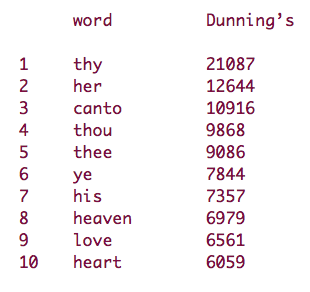
But there’s a problem with this measure, as Adam Kilgarriff has pointed out (1, pp. 237-38, 247-48). A word can be common in a corpus because it’s very common in one or two works. For instance, when I characterize early-nineteenth-century poetic diction (1800-1849) by comparing a corpus of 60 volumes of poetry to a corpus of fiction, drama, and nonfiction prose from the same period (3), I get this list:

Much of this looks like “poetic diction” — but “canto” is poetic diction only in a weird sense. It happens to be very common in a few works of poetry that are divided into cantos (works for instance by Lord Byron and Walter Scott). So when everything is added up, yes, it’s more common in poetry — but it doesn’t broadly characterize the corpus. Similar problems occur for a range of other reasons (proper nouns and pronouns can be extremely common in a restricted context).

The solution Kilgarriff offers is to instead use a Mann-Whitney ranks test. This allows us to assess how consistently a given term is more common in one corpus than in another. For instance, suppose I have eight text samples of equal length. Four of them are poetry, and four are prose. I want to know whether “lamb” is significantly more common in the poetry corpus than in prose. A simple form of the Mann-Whitney test would rank these eight samples by the frequency of “lamb” and then add up their respective ranks:

Since most works of poetry “beat” most works of prose in this ranking, the sum of ranks for poetry is higher, in spite of the 31 occurrences of lamb in one work of prose — which is, let us imagine, a novel about sheep-rustling in the Highlands. But a log-likelihood test would have identified this word as more common in prose.

In reality, one never has “equal-sized” documents, but the test is not significantly distorted if one simply replaces absolute frequency with relative frequency (normalized for document size). (If one corpus has on average much smaller documents than the other does, there may admittedly be a slight distortion.) Since the number of documents in each corpus is also going to vary, it’s useful to replace the rank-sum (U) with a statistic ρ (Mann-Whitney rho) that is U, divided by the product of the sizes of the two corpora.

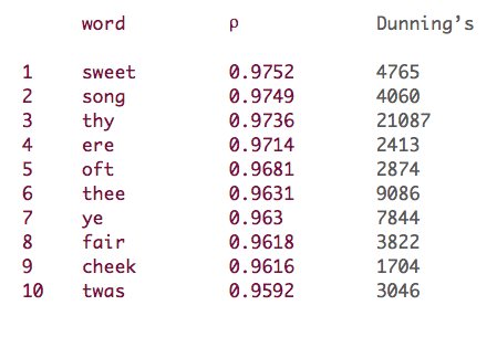
Using this measure of over-representation in a corpus produces a significantly different model of “poetic diction”:

This looks at first glance like a better model. It demotes oddities like “canto,” but also slightly demotes pronouns like “thou” and “his,” which may be very common in some works of poetry but not others. In general, it gives less weight to raw frequency, and more weight to the relative ubiquity of a term in different corpora. Kilgarriff argues that the Mann-Whitney test thereby does a better job of identifying the words that characterize male and female conversation (1, pp. 247-48).

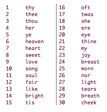
On the other hand, Paul Rayson has argued that by reducing frequency to a rank measure, this approach discards “most of the evidence we have about the distribution of words” (2). For linguists, this poses an interesting, principled dilemma, where two statistically incompatible definitions of “distinctive diction” are pitted against each other. But for a shameless literary hack like myself, it’s no trouble to cut the Gordian knot with an improvised algorithm that combines both measures. For instance, one could multiply rho by the log of Dunning’s log likelihood (represented here as G-squared) …

I don’t yet know how well this algorithm will perform if used for classification or authorship attribution. But it does produce what is for me an entirely convincing portrait of early-nineteenth-century poetic diction:

Of course, once you have an algorithm that convincingly identifies the characteristic diction of a particular genre relative to other publications in the same period, it becomes possible to say how the distinctive diction of a genre is transformed by the passage of time. That’s what I hope to address in my next post.

UPDATE Nov 10, 2011: As I continue to use these tests in different ways (using them e.g. to identify distinctively “fictional” diction, and to compare corpora separated by time) I’m finding the Mann-Whitney ρ measure more and more useful on its own. I think my urge to multiply it by Dunning’s log-likelihood may have been the needless caution of someone who’s using an unfamiliar metric and isn’t sure yet whether it will work unassisted.

References
(1) Adam Kilgarriff, “Comparing Corpora,” International Journal of Corpus Linguistics 6.1 (2001): 97-133.
(2) Paul Rayson, Matrix: A Statistical Method and Software Tool for Linguistic Analysis through Corpus Comparison. Unpublished Ph.D thesis, Lancaster University, 2003, p. 47. Cited in Magali Paquot and Yves Bestgen, “Distinctive words in academic writing: A comparison of three statistical tests for keyword extraction,” Corpora: Pragmatics and Discourse Papers from the 29th International Conference on English Language Research on Computerized Corpora (ICAME 29), Ascona, Switzerland, 14-18 May 2008, p. 254.
(3) The corpora used in this post were selected by Jordan Sellers, mostly from texts available in the Internet Archive, and corrected with a Python script described in this post.