The argument has two layers. On one level it’s about the tension between distant reading and New Historicism. The New Historical anecdote fuses history with literary representation in a vivid, influential way, by compressing a large theme into a brief episode. Can quantitative arguments about the past aspire to the same kind of compression and vividness?
Inside that metacritical frame, there’s a history of narrative pace, based on evidence I gathered in collaboration with Sabrina Lee and Jessica Mercado. (We’re also working on a separate co-authored piece that will dive more deeply into this data.)
We ask how much fictional time is narrated, on average, in 250 words. We discover some dramatic changes across a timeline of 300 years, and I’m tempted to include our results as an illustration here. But I’ve decided not to, because I want to explore whether scholars already, intuitively know how the representation of duration has changed, by asking readers to reflect for a moment on what they expect to see.
So instead of illustrating this post with real evidence, I’ve provided a plausible, counterfactual illustration based on an account of duration that one might extract from influential narratological works by Gérard Genette or Seymour Chatman.
Artificial data, generated to simulate the account of narrative pace one might extract from Gérard Genette, Narrative Discourse. Logarithmic scale.
Literary critics have been having a speculative conversation about close and distant reading. It might be premature to call it a debate.
A “debate” is normally a situation where people are free to choose between two paths. “Should I believe Habermas, or Foucault? I’m listening; I could go either way.” Conversation about distant reading is different, first, because there’s not much need to make a choice. Have any critics stopped reading closely? A close reading of The Bourgeois suggests that Franco Moretti hasn’t.
More importantly, this isn’t a debate yet because most of the people involved aren’t free to explore both paths. So far only a tiny number of scholars have actually tried distant reading, and it’s easy to see why. You can wake up tomorrow and try a Foucauldian reading of Frankenstein, but you can’t wake up and trace patterns of change in a thousand novels. In either case, you may need to learn new methods, but in the “distant” case, it can also take years to assemble a collection of texts.
A dataset for distant reading
To reduce barriers to entry, I’ve collaborated with HathiTrust Research Center to create an easier place to start with English-language literature. It’s aimed at scholars studying long-nineteenth-century (1750-1922) fiction and poetry, but it will gradually expand into the twentieth century. This post describes the humanistic uses of the dataset; if you want technical information, there’s more on the page where the data actually lives.
HathiTrust contains more than a million volumes in English between 1700 and 1922. Contractual agreements make it hard to share the texts themselves in bulk, but many of the questions that can be posed “at a distance” can be posed just as well using simpler representations of the texts — for instance, by counting the words they contain. To support this project, HathiTrust Research Center has extracted page-level word counts for 4.8 million volumes; scholars who are interested in the highest level of detail should go directly to their data.
However, many literary scholars are mainly concerned with books in a particular genre — they limit their inquiries, say, to “poetry” or “prose fiction.” Finding those needles in a five-millon-volume haystack is not easy. Many books in this period don’t carry genre tags; even when they do, volumes are heterogenous things. A volume of poetry, for instance, may begin with a prose life of the author and end with publishers’ ads.
The relative sizes of different genres, represented as a percentage of pages in the English-language portion of HathiTrust. 854,476 volumes are covered. Nonfiction, front matter, and back matter aren’t represented here. Results have been smoothed with a five-year moving average.
To create datasets that reliably track a single genre, we need page-level metadata. The National Endowment for the Humanities and the American Council of Learned Societies funded a year-long project to create that metadata. (The methods involved are described in a white paper on “Understanding Genre,” along with information about accuracy.) Now, by pairing this metadata with HTRC’s page-level wordcounts, I’ve created three genre-specific datasets of word counts covering poetry, fiction, and drama from 1700 to 1922. (Coverage is relatively sparse before 1750; if you need the early eighteenth century, you might want a resource like ECCO-TCP instead of or in addition to this.)
The collection consists of word counts for 101,948 volumes of fiction, 58,724 volumes of poetry, and 17,709 volumes of drama, aggregated at the volume level and including only pages identified as belonging to the relevant genre. I’ve collected these volume-level files in tar.gz chunks by genre and date, and have provided basic metadata for them all. You can use the volume IDs to view the original texts on the HathiTrust website if you need to read them closely. I’m calling this a “collection” rather than a “corpus” because I don’t necessarily recommend that you use the whole thing, as is. The whole thing may or may not represent the sample you need for your research question. What it represents is, “American university and public libraries, insofar as they were digitized in the year 2012 (when the project began).” For some big diachronic questions, that’s a good sample; for other questions, you’ll need to be more selective.
Three big blocks of stone. Like collections, these don’t represent anything in particular. But like a statue, the corpus you want to create might be contained somewhere within them.
Because this is a very large collection, it’s likely in any case that the sample you need for your research may be contained somewhere within it. To address some questions, you might even select several samples and contrast them. To understand the history of literary prestige, for instance, Jordan Sellers and I gathered 360 prominent books of poetry by finding reviews in literary magazines and extracting the corresponding books from HathiTrust; we then contrasted that to a sample of 360 more obscure volumes selected from the whole HathiTrust collection of poetry. Just using volume-level wordcounts for those two samples, we were able to draw inferences about the way diachronic literary change is related to synchronic prestige.
Well-known texts may be represented in this dataset by dozens of reprints. For some questions, that may be exactly the sort of “weighted” sample you want; for other questions, you’ll want to winnow each title down to a single early example. More datasets may be developed to help you do that.
Distant reading rarely means “big data”
I realize the practice described above (selecting samples of a few hundred or a few thousand books to address particular questions) doesn’t line up with the version of distant reading currently circulating in public imagination. Isn’t the point of distant reading to construct a massive database that includes “everything that has been thought and said”?The Nation recently said so, and also warned us that “in reality, servers powerful enough to process big data can only be located in a highly select number of well-endowed institutions.”
That sounds grim, but I’m happy to report that it’s also malarkey. You can download this dataset, and process it, on your laptop. It’s true that I used our campus cluster to create it (because I had to manage a terabyte of text). But a) managing a terabyte won’t put a hole in most endowments, and b) you don’t need to do that anyway. Once nonfiction is set aside, we’re talking about a smaller group of books (compressed, this whole dataset runs to about 5GB). A well-designed sampling strategy can make it even smaller.
Wait, what’s this about “sampling”? aren’t distant readers supposed to claim to have everything? Not really. In the early days of distant reading, Franco Moretti did frame the project as a challenge to literary historians’ claims about synchronic coverage. (We only discuss a tiny number of books from any given period — what about all the rest?) But even in those early publications, Moretti acknowledged that we would only be able to represent “all the rest” through some kind of sample.
Fifteen years later, it’s becoming clear that distant reading has a lot of applications that aren’t about synchronic completeness at all. Expanding the diachronic scope of our research can be an equally important source of discovery. Certain kinds of change only become visible when you compare many examples across long timelines. Even if we restricted a digital corpus (say) to the academic canon, or to a thousand bestsellers, computational analysis would allow us to see long-term changes that aren’t visible to casual recollection.
It’s true that distant readers will often want to have the biggest possible table of metadata, so that our sampling strategies aren’t unduly constrained. But from that table, we may only sample a few hundred or a few thousand titles to address any single question. This scale of inquiry is not, in any meaningful sense, “big data.” (In fact, I doubt the phrase “big data” is often very meaningful, but that’s another story.) It’s a larger sample than literary scholars have usually attempted to describe, but it would not greatly distress our neighbors in linguistics and sociology.
How hard is this to use?
Of course, we’re not linguists or sociologists, so there is going to be a learning curve involved when we apply quantitative methods on any scale. The main dataset I’m providing here includes 178,381 separate files — one file for each volume. This is not something that can be sliced easily using a tool like Excel. Someone involved with the project needs to be able to program in order to pair the metadata table with the files.
On the other hand, there may be some questions that can be answered with a simple yearly summary, so I’ve also provided yearly_summary tables for each genre that aggregate term frequencies for the 10,000 most common tokens in each genre (selected by document frequency). This is the gentlest on-ramp to the dataset; data in this form probably can be sliced with Excel; to make it even easier I’ve also gone ahead and applied OCR correction and spelling normalization to those tables.
But the yearly_summary table aggregates all the volumes in the collection, and (as I’ve stressed) you may not want all of them. This dataset is a roughly-hewn, but very large, block of stone. You may be able to find the corpus you need somewhere within it, but decisions about selection are yours to make. Over the course of the next two years I hope to extend coverage further into the twentieth century; it is not illegal to share word counts from texts still covered by copyright. If you’re interested in more complex kinds of distant reading where word order matters, you can contact the HathiTrust Research Center; they are creating a workflow that can handle more complex kinds of computational analysis.
Postscript: We’ve done a lot of testing, but this is still a beta release. General estimates about error are summarized in “Understanding Genre”. Precision in these datasets is higher than 97%, but that still means there will be hundreds of volumes and thousands of pages mistakenly included. If you notice systematic problems with the data, please send feedback to the e-mail address provided in the data description. But individual misclassified volumes are not problems we’re likely to fix on a case-by-case basis; that sort of problem will be addressed by improving our methods in our next release.
The relative sizes of different genres, represented as a percentage of pages in the English-language portion of HathiTrust. 854,476 volumes are covered. Nonfiction, front matter, and back matter aren't represented here. Results have been smoothed with a five-year moving average.
Although methods of analysis are more fun to discuss, the most challenging part of distant reading may still be locating the texts in the first place [1].
In principle, millions of books are available in digital libraries. But literary historians need collections organized by genre, and locating the fiction or poetry in a digital library is not as simple as it sounds. Older books don’t necessarily have genre information attached. (In HathiTrust, less than 40% of English-language fiction published before 1923 is tagged “fiction” in the appropriate MARC control field.)
Volume-level information wouldn’t be enough to guide machine reading in any case, because genres are mixed up inside volumes. For instance Hoyt Long, Richard So, and I recently published an article in Slate arguing (among other things) that references to specific amounts of money become steadily more common in fiction from 1825 to 1950.
Frequency of reference to “specific amounts” of money in 7,700 English-language works of fiction. Graphics here and throughout from Wickham, ggplot2 [2].
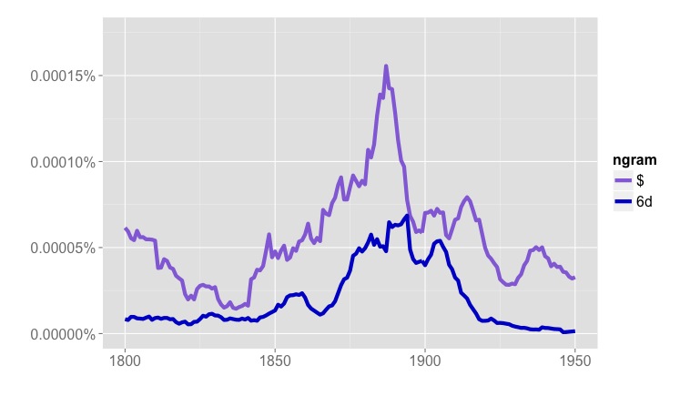
But Google’s “English Fiction” collection tells a very different story. The frequencies of many symbols that appear in prices (dollar signs, sixpence) skyrocket in the late nineteenth century, and then drop back by the early twentieth.
Frequencies of “$” and “6d” in Google’s “English Fiction” collection, 1800-1950.
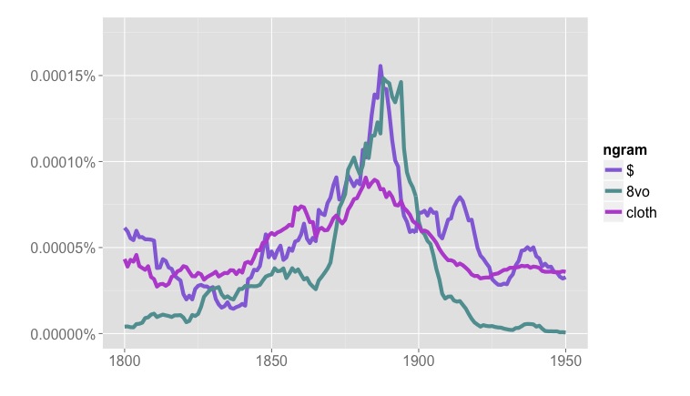
Frequencies of “$”, “8vo” (octavo) and “cloth” in Google’s “English Fiction” collection, 1800-1950.
What we see in Google’s “Fiction” collection is something that happens in volumes of fiction, but not exactly in the genre of fiction — the rise and fall of publishers’ catalogs in the backs of books [3]. Individually, these two- or three-page lists of titles for sale may not look like significant noise, but because they often mention prices, and are distributed unevenly across the timeline, they add up to a significant potential pitfall for anyone interested in the role of money in fiction.
I don’t say this to criticize the team behind the Ngram Viewer. Genre wasn’t central to their goals; they provided a rough “fiction” collection merely as a cherry on top of a massively successful public-humanities project. My point is just that genres fail to line up with volume boundaries in ways that can really matter for the questions scholars want to pose. (In fact, fiction may be the genre that comes closest to lining up with volume boundaries: drama and poetry often appear mixed in The Collected Poems and Plays of So-and-So, With a Prose Life of the Author.)
You can solve this problem by selecting works manually, or by borrowing proprietary collections from a vendor. Those are both good, practical solutions, especially up to (say) 1900. But because they rely on received bibliographies, they may not entirely fulfill the promises we’ve been making about dredging the depths of “the great unread,” boldly going where no one has gone before, etc [4]. Over the past two years, with support from the ACLS and NEH, I’ve been trying to develop another alternative — a way of starting with a whole library, and dividing it by genre at the page level, using machine learning.
In researching the Slate article, we relied on that automatic mapping of genre to select pages of fiction from HathiTrust. It helped us avoid conflating advertisements with fiction, and I hope other scholars will also find that it reduces the labor involved in creating large, genre-specific collections. The point of this blog post is to announce the release of a first version of the map we used (covering 854,476 English-language books in HathiTrust 1700-1922).
We identify pages as paratext (front matter, back matter, ads), prose nonfiction, poetry (narrative and lyric are grouped together), drama (including verse drama), or prose fiction. The report discusses the rationale for these choices, but other choices would be possible.
“How accurate is this map?”
Since genres are social institutions, questions about accuracy are relative to human dissensus. Our pairs of human readers agreed about the five categories just mentioned for 94.5% of the pages they tagged [5]. Relying on two-out-of-three voting (among other things), we boiled those varying opinions down to a human consensus, and our model agreed with the consensus 93.6% of the time. So this map is nearly as accurate as we might expect crowdsourcing to be. But it covers 276 million pages. For full details, see the confusion matrices in the report. Also, note that we provide ways of adjusting the tradeoff between recall and precision to fit a researcher’s top priority — which could be catching everything that might belong in a genre, or filtering out everything that doesn’t belong. We provide filtered collections of drama, fiction, and poetry for scholars who want to work with datasets that are 97-98% precise.
The short answer: we can’t. I don’t expect the genre predictions in this dataset to be more than one resource among many. We’ve also designed this dataset to have a certain amount of flexibility. There are confidence metrics associated with each volume, and users can define their collection of, say, poetry more broadly or narrowly by adjusting the confidence thresholds for inclusion. So even this dataset is not really a single map.
“What about divisions below the page level?”
With the exception of divisions between running headers and body text, we don’t address them. There are certainly a wide range of divisions below the page level that can matter, but we didn’t feel there was much to be gained by trying to solve all those problems at the same time as page-level mapping. In many cases, divisions below the page level are logically a subsequent step.
“How would I actually use this map to find stuff?”
There are three different ways — see “How to use this data?” in the interim report. If you’re working with HathiTrust Research Center, you could use this data to define a workset in their portal. Alternatively, if your research question can be answered with word frequencies, you could download public page-level features from HTRC and align them with our genre predictions on your own machine to produce a dataset of word counts from “only pages that have a 97% probability of being prose fiction,” or what have you. (HTRC hasn’t released feature counts for all the volumes we mapped yet, but they’re about to.) You can also align our predictions directly with HathiTrust zip files, if you have those. The pagealigner module in the utilities subfolder of our Github repo is intended as a handy shortcut for people who use Python; it will work both with HT zip files and HTRC feature files, aligning them with our genre predictions and returning a list of pages zipped with genre codes.
Is this sort of collection really what I need for my project?
Maybe not. There are a lot of books in HathiTrust. But as I admitted in my last post, a medium-sized collection based on bibliographies may be a better starting point for most scholars. Library-based collections include things like reprints, works in translation, juvenile fiction, and so on, that could be viewed as giving a fuller picture of literary culture … or could be viewed as messy complicating factors. I don’t mean to advocate for a library-based approach; I’m just trying to expand the range of alternatives we have available.
“What if I want to find fiction in French books between 1900 and 1970?”
Although we’ve made our code available as a resource, we definitely don’t want to represent it as a “tool” that could simply be pointed at other collections to do the same kind of genre mapping. Much of the work involved in this process is domain-specific (for instance, you have to develop page-level training data in a particular language and period). So this is better characterized as a method than a tool, and the report is probably more important than the repo. I plan to continue expanding the English-language map into the twentieth century (algorithmic mapping of genre may in fact be especially necessary for distant reading behind the veil of copyright). But I don’t personally have plans to expand this map to other languages; I hope someone else will take up that task.
As a reward for reading this far, here’s a visualization of the relative sizes of genres across time, represented as a percentage of pages in the English-language portion of HathiTrust.
The relative sizes of different genres, represented as a percentage of pages in the English-language portion of HathiTrust. 854,476 volumes are covered. Nonfiction, front matter, and back matter aren’t represented here. Results have been smoothed with a five-year moving average. Click through to enlarge.
The blog post above often slips awkwardly into first-person plural, because I’m describing a project that involved a lot of people. Parts of the code involved were written by Michael L. Black and Boris Capitanu. The code also draws on machine learning libraries in Weka and Scikit-Learn [6, 7]. Shawn Ballard organized the process of gathering training data, assisted by Jonathan Cheng, Nicole Moore, Clara Mount, and Lea Potter. The project also depended on collaboration and conversation with a wide range of people at HathiTrust Digital Library, HathiTrust Research Center, and the University of Illinois Library, including but not limited to Loretta Auvil, Timothy Cole, Stephen Downie, Colleen Fallaw, Harriett Green, Myung-Ja Han, Jacob Jett, and Jeremy York. Jana Diesner and David Bamman offered useful advice about machine learning. Essential material support was provided by a Digital Humanities Start-Up Grant from the National Endowment for the Humanities and a Digital Innovation Fellowship from the American Council of Learned Societies. None of these people or agencies should be held responsible for mistakes.
References
[1] Perhaps it goes without saying, since the phrase has now lost its quotation marks, but “distant reading” is Franco Moretti, “Conjectures on World Literature,” New Left Review 1 (2000).
[2] Hadley Wickham, ggplot2: Elegant Graphics for Data Analysis.http: //had.co.nz/ggplot2/book. Springer New York, 2009.
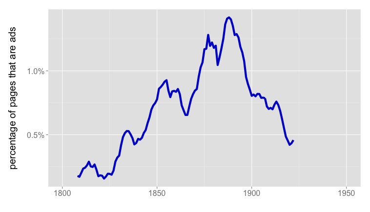
[3] Having mapped advertisements in volumes of fiction, I’m pretty certain that they’re responsible for the spike in dollar signs in Google’s “English Fiction” collection. The collection I mapped overlaps heavily with Google Books, and the number of pages of ads in fiction volumes tracks very closely with the frequency of dollars signs, “8vo,” and so on.
Percentage of pages in mostly-fiction volumes that are ads. Based on a filtered collection of 102,349 mostly-fiction volumes selected from a larger group of 854,476 volumes 1700-1922. Five-year moving average.
[4] “The great unread” comes from Margaret Cohen, The Sentimental Education of the Novel (Princeton NJ: Princeton University Press, 1999), 23.
[5] See the interim report (subsection, “Evaluating Confusion Matrices”) for a fuller description; it gets complicated, because we actually assessed accuracy in terms of the number of words misclassified, although the classification was taking place at a page level.
[6] F. Pedregosa, G. Varoquaux, A. Gramfort, V. Michel, B. Thirion, O. Grisel, M. Blondel, P. Prettenhofer, R. Weiss, V. Dubourg, J. Vanderplas, A. Passos, D. Cournapeau, M. Brucher, M. Perrot, and E. Duchesnay. Scikit-learn: Machine learning in Python. Journal of Machine Learning Research, 12:2825–2830, 2011.
[7] Mark Hall, Eibe Frank, Geoffrey Holmes, Bernhard Pfahringer, Peter Reutemann, and Ian H. Witten. The WEKA data mining software: An update. SIGKDD Explorations, 11(1), 2009.
There are basically two different ways to build collections for distant reading. You can build up collections of specific genres, selecting volumes that you know belong to them. Or you can take an entire digital library as your base collection, and subdivide it by genre.
Most people do it the first way, and having just spent two years learning to do it the second way, I’d like to admit that they’re right. There’s a lot of overhead involved in mining a library. The problem becomes too big for your desktop; you have to schedule batch jobs; you have to learn to interpret MARC records. All this may be necessary eventually, but it’s not the ideal place to start.
But some of the problems I’ve encountered have been interesting. In particular, the problem of “dividing a library by genre” has made me realize that literary studies is constituted by exclusions that are a bit larger and more arbitrary than I used to think.
First of all, why is dividing by genre even a problem? Well, most machine-readable catalog records don’t say much about genre, and even if they did, a single volume usually contains multiple genres anyway. (Think introductions, indexes, collected poems and plays, etc.) With support from the ACLS and NEH, I’ve spent the last year wrestling with that problem, and in a couple of weeks I’m going to share an imperfect page-level map of genre for English-language books in HathiTrust 1700-1923.
But the bigger thing I want to report is that the ambiguity of genre may run deeper than most scholars who aren’t librarians currently imagine. To be sure, we know that subgenres like “detective fiction” are social institutions rather than natural forms. And in a vague way we also accept that broader categories like “fiction” and “poetry” are social constructs with blurry edges. We can all point to a few anomalies: prose poems, eighteenth-century journalistic fictions like The Spectator, and so on.
But somehow, in spite of knowing this for twenty years, I never grasped the full scale of the problem. For instance, I knew the boundary between fiction and nonfiction was blurry in the 18c, but I thought it had stabilized over time. By the time you got to the Victorians, surely, you could draw a circle around “fiction.” Exceptions would just prove the rule.
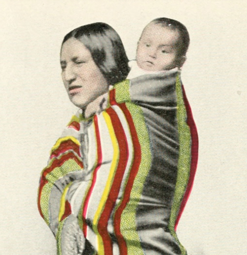
Selecting volumes one by one for genre-specific collections didn’t shake my confidence. But if you start with a whole library and try to winnow it down, you’re forced to consider a lot of things you would otherwise never look at. I’ve become convinced that the subset of genre-typical cases (should we call them cis-genred volumes?) is nowhere near as paradigmatic as literary scholars like to imagine. A substantial proportion of the books in a library don’t fit those models. This is both a photograph of a real, unnamed mother and baby, and a picture of a fictional character named Shinkah. Frontispiece to Shinkah, The Osage Indian (1916).
Consider the case of Shinkah, the Osage Indian, published in 1916 by S. M. Barrett. The preface to this volume informs us that it’s intended as a contribution to “the sociology of the Osage Indians.” But it’s set a hundred years in the past, and the central character Shinkah is entirely fictional (his name just means “child.”) On the other hand, the book is illustrated with photographs of real contemporary people, who stand for the characters in an ethnotypical way.
After wading though 872,000 volumes, I’m sorry to report that odd cases of this kind are more typical of nineteenth- and early twentieth-century fiction than my graduate-school training had led me to believe. There’s a smooth continuum for instance between Shinkah and Old Court Life in France (1873), by Frances Elliot. This book has a bibliography, and a historiographical preface, but otherwise reads like a historical novel, complete with invented dialogue. I’m not sure how to distinguish it from other historical novels with real historical personages as characters.
Literary critics know there’s a problem with historical fiction. We also know about the blurry boundary between fiction, journalism, and travel writing represented by the genre of the “sketch.” And anyone who remembers James Frey being kicked out of Oprah Winfrey’s definition of nonfiction knows that autobiographies can be problematic. And we know that didactic fiction blurs into philosophical dialogue. And anyone who studies children’s literature knows that the boundary between fiction and nonfiction gets especially blurry there. And probably some of us know about ethnographic novels like Shinkah. But I’m not sure many of us (except for librarians) have added it all up. When you’re sorting through an entire library you’re forced to see the scale of it: in the period 1700-1923, maybe 10% of the volumes that could be cataloged as fiction present puzzling boundary cases.
You run into a lot of these works even if you browse or select titles at random; that’s how I met Shinkah. But I’ve also been training probabilistic models of genre that report, among other things, how certain or uncertain they are about each page. These models are good at identifying clear cases of our received categories; I found that they agreed with my research assistants almost exactly as often as the research assistants agreed with each other (93-94% of the time, about broad categories like fiction/nonfiction). But you can also ask a model to sift through several thousand volumes looking for hard cases. When I did that I was taken aback to discover that about half the volumes it had most trouble with were things I also found impossible to classify. The model was most uncertain, for instance, about The Terrific Register (1825) — an almanac that mixes historical anecdote, urban legend, and outright fiction randomly from page to page. The second-most puzzling book was Madagascar, or Robert Drury’s Journal (1729), a book that offers itself as a travel journal by a real person, and was for a long time accepted as one, although scholars have more recently argued that it was written by Defoe.
Of course, a statistical model of fiction doesn’t care whether things “really happened”; it pays attention mostly to word frequency. Past-tense verbs of speech, personal names, and “the,” for instance, are disproportionately common in fiction. “Is” and “also” and “mr” (and a few hundred other words) are common in nonfiction. Human readers probably think about genre in a more abstract way. But it’s not particularly miraculous that a model using word frequencies should be confused by the same examples we find confusing. The model was trained, after all, on examples tagged by human beings; the whole point of doing that was to reproduce as much as possible the contours of the boundary that separates genres for us. The only thing that’s surprising is that trawling the model through a library turns up more books right in the middle of the boundary region than our habits of literary attention would have suggested.
A lot of discussions of distant reading have imagined it as a move from canonical to popular or obscure examples of a (known) genre. But reconsidering our definitions of the genres we’re looking for may be just as important. We may come to recognize that “the novel” and “the lyric poem” have always been islands floating in a sea of other texts, widely read but never genre-typical enough to be replicated on English syllabi.
In the long run, this may require us to balance two kinds of inclusiveness. We already know that digital libraries exclude a lot. Allen Riddell has nicely demonstrated just how much: he concludes that there are digital scans for only about 58% of the novels listed in bibliographies as having been published between 1800 and 1836.
One way to ensure inclusion might be to start with those bibliographies, which highlight books invisible in digital libraries. On the other hand, bibliographies also make certain things invisible. The Terrific Register (1825), for instance, is not in Garside’s bibliography of early-nineteenth-century fiction. Neither is The Wonder-Working Water Mill (1791), to mention another odd thing I bumped into. These aren’t oversights; Garside et. al. acknowledge that they’re excluding certain categories of fiction from their conception of the novel. But because we’re trained to think about novels, the scale of that exclusion may only become visible after you spend some time trawling a library catalog.
I don’t want to present this as an aporia that makes it impossible to know where to start. It’s not. Most people attempting distant reading are already starting in the right place — which is to build up medium-sized collections of familiar generic categories like “the novel.” The boundaries of those categories may be blurrier than we usually acknowledge. But there’s also such a thing as fretting excessively about the synchronic representativeness of your sample. A lot of the interesting questions in distant reading are actually trends that involve relative, diachronic differences in the collection. Subtle differences of synchronic coverage may more or less drop out of questions about change over time.
On the other hand, if I’m right that the gray areas between (for instance) fiction and nonfiction are bigger and more persistently blurry than literary scholarship usually mentions, that’s probably in the long run an issue we should consider! When I release a page-level map of genre in a couple of weeks, I’m going to try to provide some dials that allow researchers to make more explicit choices about degrees of inclusion or exclusion.
Predictive models that report probabilities give us a natural way to handle this, because they allow us to characterize every boundary as a gradient, and explicitly acknowledge our compromises (for instance, trade-offs between precision and recall). People who haven’t done much statistical modeling often imagine that numbers will give humanists spuriously clear definitions of fuzzy concepts. My experience has been the opposite: I think our received disciplinary practices often make categories seem self-evident and stable because they teach us to focus on easy cases. Attempting to model those categories explicitly, on a large scale, can force you to acknowledge the real instability of the boundaries involved.
References and acknowledgments
Training data for this project was produced by Shawn Ballard, Jonathan Cheng, Lea Potter, Nicole Moore and Clara Mount, as well as me. Michael L. Black and Boris Capitanu built a GUI that helped us tag volumes at the page level. Material support was provided by the National Endowment for the Humanities and the American Council of Learned Societies. Some information about results and methods is online as a paper and a poster, but much more will be forthcoming in the next month or so — along with a page-level map of broad genre categories and types of paratext.
The project would have been impossible without help from HathiTrust and HathiTrust Research Center. I’ve also been taught to read MARC records by librarians and information scientists including Tim Cole, M. J. Han, Colleen Fallaw, and Jacob Jett, any of whom could teach a course on “Cursed Metadata in Theory and Practice.”
I mention Garside’s bibliography of early nineteenth-century fiction. This is Garside, Peter, and Rainer Schöwerling. The English novel, 1770-1829 : a bibliographical survey of prose fiction published in the British Isles. Ed. Peter Garside, James Raven, and Rainer Schöwerling. 2 vols. Oxford: Oxford University Press, 2000.
The Institute of Electrical and Electronics Engineers is an odd venue for literary history, and our paper ends up touching so many disciplinary bases that it may be distracting.* So I thought I’d pull out four issues of interest to humanists and discuss them briefly here; I’m also taking the occasion to add a little information about gender that we uncovered too late to include in the paper itself.
1) The overall point about genre. Our title, “Mapping Mutable Genres in Structurally Complex Volumes,” may sound like the sort of impossible task heroines are assigned in fairy tales. But the paper argues that the blurry mutability of genres is actually a strong argument for a digital approach to their history. If we could start from some consensus list of categories, it would be easy to crowdsource the history of genre: we’d each take a list of definitions and fan out through the archive. But centuries of debate haven’t yet produced stable definitions of genre. In that context, the advantage of algorithmic mapping is that it can be comprehensive and provisional at the same time. If you change your mind about underlying categories, you can just choose a different set of training examples and hit “run” again. In fact we may never need to reach a consensus about definitions in order to have an interesting conversation about the macroscopic history of genre.
2) A workset of 32,209 volumes of English-language fiction. On the other hand, certain broad categories aren’t going to be terribly controversial. We can probably agree about volumes — and eventually specific page ranges — that contain (for instance) prose fiction and nonfiction, narrative and lyric poetry, and drama in verse, or prose, or some mixture of the two. (Not to mention interesting genres like “publishers’ ads at the back of the volume.”) As a first pass at this problem, we extract a workset of 32,209 volumes containing prose fiction from a collection of 469,200 eighteenth- and nineteenth-century volumes in HathiTrust Digital Library. The metadata for this workset is publicly available from Illinois’ institutional repository. More substantial page-level worksets will soon be produced and archived at HathiTrust Research Center.
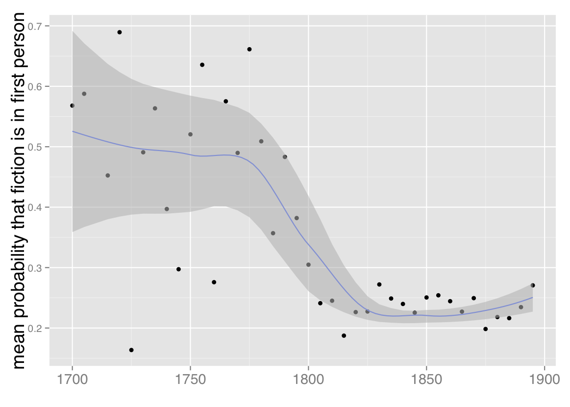
3) The declining prevalence of first-person narration. Once we’ve identified this fiction workset, we switch gears to consider point of view — frankly, because it’s a temptingly easy problem with clear literary significance. Though the fiction workset we’re using is defined more narrowly than it was last February, we confirm the result I glimpsed at that point, which is that the prevalence of first-person point of view declines significantly toward the end of the eighteenth century and then remains largely stable for the nineteenth.
Mean probability that fiction is written in first person, 1700-1899. Based on a corpus of 32,209 volumes of fiction extracted from HathiTrust Digital Library. Points are mean probabilities for five-year spans of time; a trend line with standard errors has been plotted with loess smoothing.
We can also confirm that result in a way I’m finding increasingly useful, which is to test it in a collection of a completely different sort. The HathiTrust collection includes reprints, which means that popular works have more weight in the collection than a novel printed only once. It also means that many volumes carry a date much later than their first date of publication. In some ways this gives a more accurate picture of print culture (an approximation to “what everyone read,” to borrow Scott Weingart’s phrase), but one could also argue for a different kind of representativeness, where each volume would be included only once, in a record dated to its first publication (an attempt to represent “what everyone wrote”).
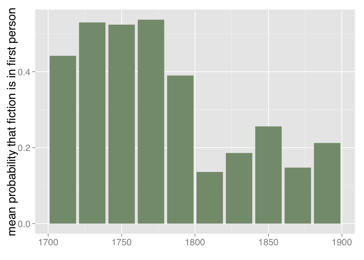
Mean probability that fiction is written in first person, 1700-1899. Based on a corpus of 774 volumes of fiction selected by multiple hands from multiple sources. Plotted in 20-year bins because n is smaller here. Works are weighted by the number of words they contain.
Fortunately, Jordan Sellers and I produced a collection like that a few years ago, and we can run the same point-of-view classifier on this very different set of 774 fiction volumes (metadata available), selected by multiple hands from multiple sources (including TCP-ECCO, the Brown Women Writers Project, and the Internet Archive). Doing that reveals broadly the same trend line we saw in the HathiTrust collection. No collection can be absolutely representative (for one thing, because we don’t agree on what we ought to be representing). But discovering parallel results in collections that were constructed very differently does give me some confidence that we’re looking at a real trend.
4. Gender and point of view. In the process of classifying works of fiction, we stumbled on interesting thematic patterns associated with point of view. Features associated with first-person perspective include first-person pronouns, obviously, but also number words and words associated with sea travel. Some of this association may be explained by the surprising persistence of a particular two-century-long genre, the Robinsonade. A castaway premise obviously encourages first-person narration, but the colonial impulse in the Robinsonade also seems to have encouraged acquisitive enumeration of the objects (goats, barrels, guns, slaves) its European narrators find on ostensibly deserted islands. Thus all the number words. (But this association of first-person perspective with colonial settings and acquisitive enumeration may well extend beyond the boundaries of the Robinsonade to other genres of adventure fiction.)
Third-person perspective, on the other hand, is durably associated with words for domestic relationships (husband, lover, marriage). We’re still trying to understand these associations; they could be consequences of a preference for third-person perspective in, say, courtship fiction. But third-person pronouns correlate particularly strongly with words for feminine roles (girl,daughter,woman) — which suggests that there might also be a more specifically gendered dimension to this question.
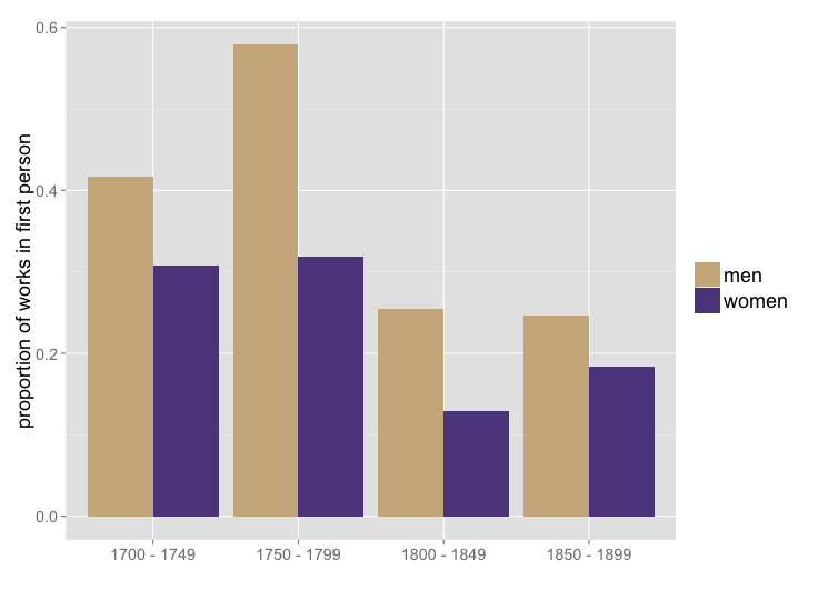
Since transmitting our paper to the IEEE I’ve had a chance to investigate this hypothesis in the smaller of the two collections we used for that paper — 774 works of fiction between 1700 and 1899: 521 by men, 249 by women, and four not characterized by gender. (Mike Black and Jordan Sellers recorded this gender data by hand.) In this collection, it does appear that male writers choose first-person perspective significantly more than women do. The gender gap persists across the whole timespan, although it might be fading toward the end of the nineteenth century.
Proportion of works of fiction by men and women in first person. Based on the same set of 774 volumes described above. (This figure counts strictly by the number of works rather than weighting works by the number of words they contain.)
Over the whole timespan, women use first person in roughly 23% of their works, and men use it in roughly 35% of their works.** That’s not a huge difference, but in relative terms it’s substantial. (Men are using first person 52% more than women). The Bayesian mafia have made me wary of p-values, but if you still care: a chi-squared test on the 2×2 contingency table of gender and point of view gives p < 0.001. (Attentive readers may already be wondering whether the decline of first person might be partly explained by an increase in the proportion of women writers. But actually, in this collection, works by women have a distribution that skews slightly earlier than that of works by men.)
These are very preliminary results. 774 volumes is a small set when you could test 32,209. At the recent HTRC Uncamp, Stacy Kowalczyk described a method for gender identification in the larger HathiTrust corpus, which we will be eager to borrow once it’s published. Also, the mere presence of an association between gender and point of view doesn’t answer any of the questions literary critics will really want to pose about this phenomenon — like, why is point of view associated with gender? Is this actually a direct consequence of gender, or is it an indirect consequence of some other variable like genre? Does this gendering of narrative perspective really fade toward the end of the nineteenth century? I don’t pretend to have answered any of those questions, all I’m doing here is flagging the existence of an interesting open question that will deserve further inquiry.
** We don’t actually represent point of view as a binary choice between first person or third person; the classifier reports probabilities as a continuous range between 0 and 1. But for purposes of this blog post I’ve simplified by dividing the works into two sets at the 0.5 mark. On this point, and for many other details of quantitative methodology, you’ll want to consult the paper itself.
Digital collections are vastly expanding literary scholars’ field of view: instead of describing a few hundred well-known novels, we can now test our claims against corpora that include tens of thousands of works. But because this expansion of scope has also raised expectations, the question of representativeness is often discussed as if it were a weakness rather than a strength of digital methods. How can we ever produce a corpus complete and balanced enough to represent print culture accurately?
I think the question is wrongly posed, and I’d like to suggest an alternate frame. As I see it, the advantage of digital methods is that we never need to decide on a single model of representation. We can and should keep enlarging digital collections, to make them as inclusive as possible. But no matter how large our collections become, the logic of representation itself will always remain open to debate. For instance, men published more books than women in the eighteenth century. Would a corpus be correctly balanced if it reproduced those disproportions? Or would a better model of representation try to capture the demographic reality that there were roughly as many women as men? There’s something to be said for both views.
To take another example, Scott Weingart has pointed out that there’s a basic tension in text mining between measuring “what was written” and “what was read.” A corpus that contains one record for every title, dated to its year of first publication, would tend to emphasize “what was written.” Measuring “what was read” is harder: a perfect solution would require sales figures, reviews, and other kinds of evidence. But, as a quick stab at the problem, we could certainly measure “what was printed,” by including one record for every volume in a consortium of libraries like HathiTrust. If we do that, a frequently-reprinted work like Robinson Crusoe will carry about a hundred times more weight than a novel printed only once.
We’ll never create a single collection that perfectly balances all these considerations. But fortunately, we don’t need to: there’s nothing to prevent us from framing our inquiry instead as a comparative exploration of many different corpora balanced in different ways.
For instance, if we’re troubled by the difference between “what was written” and “what was read,” we can simply create two different collections — one limited to first editions, the other including reprints and duplicate copies. Neither collection is going to be a perfect mirror of print culture. Counting the volumes of a novel preserved in libraries is not the same thing as counting the number of its readers. But comparing these collections should nevertheless tell us whether the issue of popularity makes much difference for a given research question.
I suspect in many cases we’ll find that it makes little difference. For instance, in tracing the development of literary language, I got interested in the relative prominence of words that entered English before and after the Norman Conquest — and more specifically, in how that ratio changed over time in different genres. My first approach to this problem was based on a collection of 4,275 volumes that were, for the most part, limited to first editions (773 of these were prose fiction).
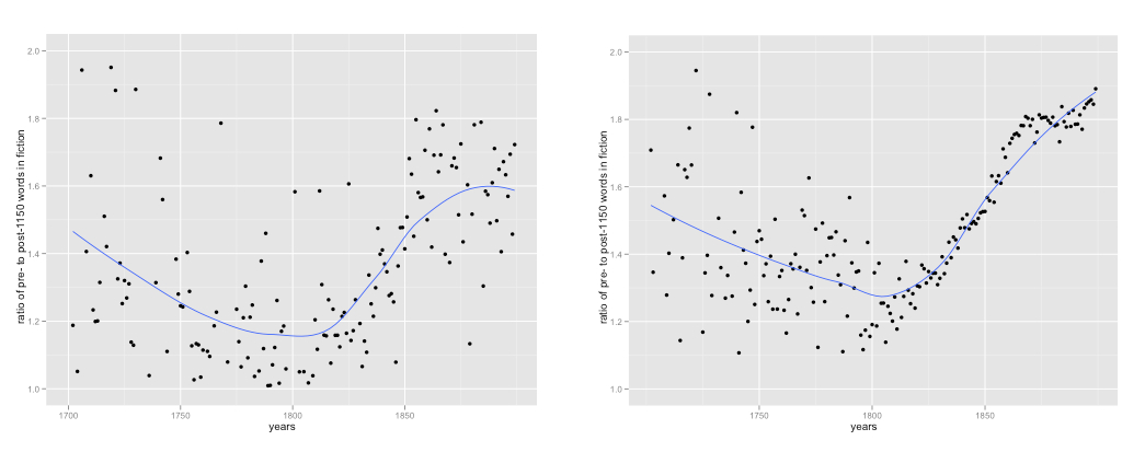
But I recognized that other scholars would have questions about the representativeness of my sample. So I spent the last year wrestling with 470,000 volumes from HathiTrust; correcting their OCR and using classification algorithms to separate fiction from the rest of the collection. This produced a collection with a fundamentally different structure — where a popular work of fiction could be represented by dozens or scores of reprints scattered across the timeline. What difference did that make to the result? (click through to enlarge) The same question posed to two different collections. 773 hand-selected first editions on the left; on the right, 47,549 volumes, including many translations and reprints. Yearly ratios are plotted rather than individual works.
It made almost no difference. The scatterplots look different, of course, because the hand-selected collection (on the left) is relatively stable in size across the timespan, and has a consistent kind of noisiness, whereas the HathiTrust collection (on the right) gets so huge in the nineteenth century that noise almost disappears. But the trend lines are broadly comparable, although the collections were created in completely different ways and rely on incompatible theories of representation.
I don’t regret the year I spent getting a binocular perspective on this question. Although in this case changing the corpus made little difference to the result, I’m sure there are other questions where it will make a difference. And we’ll want to consider as many different models of representation as we can. I’ve been gathering metadata about gender, for instance, so that I can ask what difference gender makes to a given question; I’d also like to have metadata about the ethnicity and national origin of authors.
But the broader point I want to make here is that people pursuing digital research don’t need to agree on a theory of representation in order to cooperate.
If you’re designing a shared syllabus or co-editing an anthology, I suppose you do need to agree in advance about the kind of representativeness you’re aiming to produce. Space is limited; tradeoffs have to be made; you can only select one set of works.
But in digital research, there’s no reason why we should ever have to make up our minds about a model of representativeness, let alone reach consensus. The number of works we can select for discussion is not limited. So we don’t need to imagine that we’re seeking a correspondence between the reality of the past and any set of works. Instead, we can look at the past from many different angles and ask how it’s transformed by different perspectives. We can look at all the digitized volumes we have — and then at a subset of works that were widely reprinted — and then at another subset of works published in India — and then at three or four works selected as case studies for close reading. These different approaches will produce different pictures of the past, to be sure. But nothing compels us to make a final choice among them.
This post is an outline of discussion topics I’m proposing for a workshop at NASSR2012 (a conference of Romanticists). I’m putting it on the blog since some of the links might be useful for a broader audience.
In the morning I’ll give a few examples of concrete literary results produced by text mining. I’ll start the afternoon workshop by opening two questions for discussion: first, what are the obstacles confronting a literary scholar who might want to experiment with quantitative methods? Second, how do those methods actually work, and what are their limits?
I’ll also invite participants to play around with a collection of 818 works between 1780 and 1859, using an R program I’ve provided for the occasion. Links for these materials are at the end of this post.
I. HOW DIFFICULT IS IT TO GET STARTED?
There are two kinds of obstacles: getting the data you need, and getting the digital skills you need.
1. Is it really necessary to have a large collection of texts?
This is up for debate. But I tend to think the answer is “yes.”
Not because bigger is better, or because “distant reading” is the new hotness. It’s still true that a single passage, perceptively interpreted, may tell us more than a thousand volumes.
But if you want to interpret a single passage, you fortunately already have a wrinkled protein sponge that will do a better job than any computer. Quantitative analysis starts to make things easier only when we start working on a scale where it’s impossible for a human reader to hold everything in memory. Your mileage may vary, but I’d say, more than ten books?
And actually, you need a larger collection than that, because quantitative analysis tends to require context before it becomes meaningful. It doesn’t mean much to say that the word “motion” is common in Wordsworth, for instance, until we know whether “motion” is more common in his works than in other nineteenth-century poets. So yes, text-mining can provide clues that lead to real insights about a single author or text. But it’s likely that you’ll need a collection of several hundred volumes, for comparison, before those clues become legible.
Words that are consistently more common in works by William Wordsworth than in other poets from 1780 to 1850. I’ve used Wordle’s graphics, but the words have been selected by a Mann-Whitney test, which measures overrepresentation relative to a context — not by Wordle’s own (context-free) method. See the R script at the end of this post.
This isn’t to deny that there are interesting things that can be done digitally with a single text: digital editing, building timelines and maps, and so on. I just doubt that quantitative analysis adds much value at that scale. (And to give credit where it’s due: Mark Olsen was saying all this back in the 90s — see References.)
2. So, where do I get all those texts?
That’s what I was asking myself 18 months ago. A lot of excitement about digital humanities is premised on the notion that we already have large collections of digitized sources waiting to be used. But it’s not true, because page images are not the same thing as clean, machine-readable text.
If you’re interested in twentieth-century secondary sources, the JSTOR Data for Research API can probably get you what you need. Primary sources are a harder problem. In our own (Romantic) era, optical character recognition (OCR) is unreliable. The ratio of words transcribed accurately ranges from around 80% to around 98%, depending on print quality and typographical quirks like the notorious “long s.” For a lot of text-mining purposes, 95% might be fine, if the errors were randomly distributed. But they’re not random: errors cluster in certain words and periods.
What you see in a page image.
The problem can be addressed in several different ways. There are a few collections (like ECCO-TCP and the Brown Women Writers Project) that transcribe text manually. That’s an ideal solution, but coverage of that kind is stronger in the eighteenth than the nineteenth century.
What you may see as OCR.
So Jordan Sellers and I have supplemented those collections by automatically correcting 19c OCR that we got from the Internet Archive. Our strategy involved statistically cautious, period-specific spellchecking, combined with enough reasoning about context to realize that “mortal fin” is probably “mortal sin,” even though “fin” is a correctly spelled word. It’s not a perfect solution, but in our period it works well enough for text-mining purposes. We have corrected about 2,000 volumes this way, and are happy to share our texts and metadata, as well as the spellchecker itself (once I get it packaged well enough to distribute). I can give you either a zip file containing the 19c texts themselves, or a tab-separated file containing docIDs, words, and word counts for the whole collection. In either scheme, the docIDs are keyed to this metadata file.
Of course, selecting titles for a collection like this raises intractable questions about representativeness. We tried to maximize diversity while also selecting volumes that seemed to have reached a significant audience. But other scholars may have other priorities. I don’t think it would be useful to seek a single right answer about representativeness; instead, I’d like to see multiple scholars building different kinds of collections, making them all public, and building on each other’s work. Then we would be able to test a hypothesis against multiple collections, and see whether the obvious caveats about representativeness actually make a difference in any given instance.
3. Is it necessary to learn how to program?
I’m not going to try to answer that question, because it’s complex and better addressed through discussion.
I will tell a brief story. I went into this gig thinking that I wouldn’t have to do my own programming, since there were already public toolsets for text-mining (Voyant, MONK, MALLET, TAPoR, SEASR) and for visualization (Gephi). I figured I would just use those.
But I rapidly learned otherwise. Tools like MONK and Voyant taught me what was possible, but they weren’t well adapted for managing a very large collection of texts, and didn’t permit me to make my own methodological innovations. When you start trying to do either of those things, you rapidly need “nonstandard parts,” which means that someone in the team has to be able to program.
That doesn’t have to be a daunting prospect, because the programming involved is of a relatively forgiving sort. It’s not easy, but it’s also not professional software development. So if you want to do it yourself, that’s a plausible aspiration. Alternately, if you want to collaborate with someone, you don’t necessarily need to find “a computer scientist.” A graduate student or fellow humanist who can program will do just fine.
If you do want to learn to program, I would recommend starting with either Python or R. Of the two languages, Python is certainly easier. It’s intuitive, and well-documented, and great for working with text. If you expect to use existing tools (like MALLET), and just need some “glue” to connect them to each other, Python is probably the way to go. R is a more specialized and less intuitive language. But it happens to be specialized in some ways that are useful for text mining. In particular, it has built-in statistical functions, and a built-in plotting/graphing capacity. I’ve used it for the sample exercise that accompanies this post. But if you’re learning to program for the first time, Python might be a better all-around choice, and you could in principle extend it to do everything R does. [Later addition: You could do worse than start with The Programming Historian.]
II. WHAT CAN WE ACTUALLY DO WITH QUANTITATIVE METHODS?
What follows is just a list of elements. Interesting research projects tend to combine several of these elementary operations in ad-hoc ways suited to a particular question. The list of elements runs a little long, so let me cut to the chase: the overall theme I’m trying to convey is that you can build complex arguments on a very simple foundation. Yes, at bottom, text mining is often about counting words. But a) words matter and b) they hang together in interesting ways, like individual dabs of paint that together start to form a picture.
So, to return to the original question: what can we do?
1) Categorize documents. You can “categorize” in several different senses.
a) Information retrieval: retrieve documents that match a query. This is what you do every time you use a search engine.
b) (Supervised) classification: a program can learn to correctly distinguish texts by a given author, or learn (with a bit more difficulty) to distinguish poetry from prose, tragedies from history plays, or “gothic novels” from “sensation novels.” (See “Quantitative Formalism,” Pamphlet 1 from the Stanford Literary Lab.) The researcher has to provide examples of different categories, but doesn’t have to specify how to make the distinction: algorithms can learn to recognize a combination of features that is the “fingerprint” of a given category.
An example of clustering from “Quantitative Formalism,” Allison, Heuser, Jockers, Moretti, and Witmore, Stanford Literary Lab.
c) (Unsupervised) clustering: a program can subdivide a group of documents using general measures of similarity instead of predetermined categories. This may reveal patterns you don’t expect.
All three of these techniques can achieve amazing results armed with what seems like very crude information about the documents they’re categorizing. We know, intuitively, that merely counting words is not enough to distinguish a tragedy from a history play. But our intuitions are simply wrong — see the lit lab pamphlet I cited above. It turns out that there’s an enormous amount of information contained in relative word frequencies, even if you know nothing about sequence or syntax. As you consider other aspects of text mining, it’s useful to keep this intuitive misfire in mind. Relatively simple statistical techniques often characterize discourse a good deal better than our intuitions would predict.
2) Contrast the vocabulary of different corpora. In a way, this reverses the logic of classifying documents (1b). Instead of using features to sort documents into categories, you start with two categories of documents and contrast them to identify distinctive features.
For instance, you can discover which words (or phrases) are overrepresented in one author or genre (relative to, say, the rest of nineteenth-century literature). It can admittedly be a challenge to interpret the results: this is a kind of evidence we aren’t accustomed to yet. But lists of overrepresented words can be a fruitful source of critical leads to pursue in more traditional ways.
3) Trace the history of particular features (words or phrases) over time. This could be viewed as a special category of corpus comparison, where you’re comparing corpora segmented on the time axis.
The best-known example here would be Google’s ngram viewer. Digital humanists love to criticize the ngram viewer, partly for valid reasons (there’s no way to know what texts are being used). But it has probably been the single most influential application of text mining, so clearly people are finding this simple kind of diachronic visualization useful. A couple of other projects have built on the same dataset, slicing it in different ways. Mark Davies of BYU built an interface that lets you survey the history of collocations. Our team at Illinois built an interface that mines 18-19c correlations in the ngram dataset; it turns out that correlated words have a high likelihood of being related in other ways as well, and these can be intriguing leads: see what words correlate with “delicacy” in our period, for instance. Harvard has built Bookworm, which can be understood as a smaller but more flexible and better-documented version of the ngram viewer (built on the Open Library instead of Google Books).
Words whose frequencies correlate strongly over time are often related in other ways as well. Ngram viewer by Auvil, Capitanu, Heuser and Underwood, based on corrected Google dataset.
Of special interest to Romanticists: a project that isn’t built on the ngram dataset but that does use diachronic correlation-mining as a central methodology. In Stanford Lit Lab Pamphlet 4, Ryan Heuser and Long Le-Khac have traced some very interesting, strongly correlated changes in novelistic diction over the course of the 19th century.
Finally, anyone who wants to make a diachronic argument about diction should read Ben Schmidt’s simple, elegant experiment peeling apart two different components of change: generational succession and historical change within the diction of a single age-cohort.
4) Cluster features that tend to be associated in a given corpus of documents (aka topic modeling). In a way, this reverses the logic of clustering documents (1c). Instead of grouping documents that tend to share the same words, you group words that tend to appear in the same documents, or parts of documents. This produces something that looks like a semantic map of the period or corpus you’re studying. (It would be more accurate to call it a discursive map, because topics don’t actually have to be unified semantically. They are more analogous to “discourses.”)
There are a lot of ways to cluster features, ranging from older approaches (Latent Semantic Analysis), to the new, hip approach — “Bayesian topic modeling,” which has the advantage that it clusters individual occurrences of words (tokens) instead of word types. As a result, it can distinguish different senses of a word. (Scott Weingart has written a clear and comprehensive introduction to topic modeling for humanists.)
Topic modeling has become justifiably popular for several reasons. First and foremost, a “discursive map” can be a nice thing to have; it lends itself easily to interpretation. Also, frankly, this approach doesn’t require a whole lot of improvisation. You just pour text files into a tool like MALLET, and out come a list of topics, looking meaningful and authoritative. It’s important to remember that topic-modeling is in fact an imprecise process. Slightly different inputs (for instance, a different stopword list) can produce very different outputs.
5) Entity extraction. If you’re mainly interested in proper nouns (personal names or place names, or dates and prices) there are tools like OpenNLP that can extract these from text, using syntactic patterns as clues.
6) Visualization. Perhaps this isn’t technically a form of analysis, but in practice it’s important enough that it deserves to be treated as a separate analytical step. It’s impractical to list all possible forms of visualization here, but for instance, results can be visualized:
a) Geographically — to reflect, for instance, density of references to different parts of the world. (See
b) As a network graph — to reflect strength of affinity between different entities (characters, or topics, or what have you).
c) Through “Principal Component Analysis,” if you have multidimensional data that need to be flattened to two dimensions for ease of comprehension.
Putting things together.
There’s no limit to the number of ways you can combine these different operations. Matt Wilkens has extracted references to named entities from fiction, and then visualized their density geographically. Robert K. Nelson has performed topic modeling on the print run of a Civil-War-era newspaper, and then graphed the frequency of each topic over time. You could go a step further and look for correlations between topics (either over time, or in terms of their distribution over documents). Then you could visualize the relationships between topics as a network.
What’s the goal uniting all this experimentation? I suspect there are two different but equally valid goals. In some cases, we’re going to find patterns that actually function as evidence to support literary-historical arguments. (In a number of the examples cited above, I think that’s starting to happen.) In other cases, text mining may work mainly as an exploratory technique, revealing clues that need to be fleshed out and written up using more traditional critical methods. The boundary between those two applications will be hotly debated for years, so I won’t attempt to define it here.
III. SAMPLE DATA AND SCRIPT FOR EXPLORATION.
I don’t know whether we’ll really have time for this, but I ought to at least offer you a chance to do hands-on stuff. So here’s a medium-sized project.
Finally, I’ve provided an R script that will let you define different chunks of the collection and compare them against each other, to identify words that are significantly overrepresented in a given author, genre, or period. The script will try two different measures of “overrepresentation”: the first, “log-likelihood,” is based on the aggregate frequency of words in the corpus you selected, adding all the volumes in the corpus together. The second, “Mann-Whitney rho,” tries to locate words that are consistently more common in corpus X by paying attention to individual volumes. For more on how that works, see this blog post.
Of course, the R script won’t work until you download R and open it from within R. Please understand that this is a very rough, ad-hoc piece of work for this one occasion, not a polished piece of software that I expect people to use for the long term.
Postscript about the word “mining.”
I know it has an industrial sound; I know humanists like “analysis” more. But I’m sticking with the mining metaphor on the principle of truth in advertising. I think that word accurately conveys the scale of this enterprise, and the fact that it’s often more exploratory than probative. Besides, “mining” is vivid, and that has its own sort of humanistic value.
References (that aren’t already implicit in links)
Mark Olsen, “Signs, Symbols, and Discourses: A New Direction for Computer-Aided Literature Studies” Computers and the Humanities 27 (1993): 309-314.
I’m getting ahead of myself with this post, because I don’t have time to explain everything I did to produce this. But it was just too striking not to share.
Basically, I’m experimenting with Latent Dirichlet Allocation, and I’m impressed. So first of all, thanks to Matt Jockers, Travis Brown, Neil Fraistat, and everyone else who tried to convince me that Bayesian methods are better. I’ve got to admit it. They are.
But anyway, in a class I’m teaching we’re using LDA on a generically diverse collection of 1,853 volumes between 1751 and 1903. The collection includes fiction, poetry, drama, and a limited amount of nonfiction (just biography). We’re stumbling on a lot of fascinating things, but this was slightly moving. Here’s the graph for one particular topic.
The circles and X’s are individual volumes. Blue is fiction, green is drama, pinkish purple is poetry, black biography. Only the volumes where this topic turned out to be prominent are plotted, because if you plot all 1,853 it’s just a blurry line at the bottom of the image. The gray line is an aggregate frequency curve, which is not related in any very intelligible way to the y-axis. (Work in progress …) As you can see. this topic is mostly prominent in fiction around the year 1800. Here are the top 50 words in the topic:
But here’s what I find slightly moving. The x’s at the top of the graph are the 10 works in the collection where the topic was most prominent. They include, in order, Mary Wollstonecraft Shelley, Frankenstein, Mary Wollstonecraft, Mary, William Godwin, St. Leon, Mary Wollstonecraft Shelley, Lodore, William Godwin, Fleetwood, William Godwin, Mandeville, and Mary Wollstonecraft Shelley, Falkner.
In short, this topic is exemplified by a family! Mary Hays does intrude into the family circle with Memoirs of Emma Courtney, but otherwise, it’s Mary Wollstonecraft, William Godwin, and their daughter.
Other critics have of course noticed that M. W. Shelley writes “Godwinian novels.” And if you go further down the list of works, the picture becomes less familial (Helen Maria Williams and Thomas Holcroft butt in, as well as P. B. Shelley). Plus, there’s another topic in the model (“myself these should situation”) that links William Godwin more closely to Charles Brockden Brown than it does to his wife or daughter. And LDA isn’t graven on stone; every time you run topic modeling you’re going to get something slightly different. But still, this is kind of a cool one. “Mind feelings heart felt” indeed.
In a couple of recent posts, I argued that fiction and poetry became less similar to nonfiction prose over the period 1700-1900. But because I only measured genres’ distance from each other, I couldn’t say much substantively about the direction of change. Toward the end of the second post, though, I did include a graph that hinted at a possible cause:
The older part of the lexicon (mostly words derived from Old English) gradually became more common in poetry, fiction, and drama than in nonfiction prose. This may not be the only reason for growing differentiation between literary and nonliterary language, but it seems worth exploring. (I should note that function words are excluded from this calculation for reasons explained below; we’re talking about verbs, nouns, and adjectives — not about a rising frequency of “the.”)
Why would genres become etymologically different? Well, it appears that words of different origins are associated in contemporary English with different registers (varieties of language appropriate for a particular social situation). Words of Old English provenance get used more often in speech than in writing — and in writing they are (now) used more often in narrative than in exposition. Moreover, writers learn to produce this distinction as they get older; there isn’t a marked difference for students in elementary school. But as they advance to high school, students learn to use Latinate words in formal expository writing (Bar-Ilan and Berman, 2007).
It’s not hard to see why words of Old English origin might be associated with spoken language. English was for 200 years (1066-1250) almost exclusively spoken. The learned part of the Old English lexicon didn’t survive this period. Instead, when English began to be used again in writing, literate vocabulary was borrowed from French and Latin. As a result, etymological distinctions in English tend also to be distinctions between different social contexts of language use.
Instead of distinguishing “Germanic” and “Latinate” diction here, I have used the first attested date for each word, choosing 1150 as a dividing line because it’s the midpoint of the period when English was not used in writing. Of course pre-1150 words are mostly from Old English, but I prefer to divide based on date-of-entry because that highlights the history of writing rather than a spurious ethnic mystique. (E.g., “Anglo-Saxon is a livelier tongue than Latin, so use Anglo-Saxon words.” — E. B. White.) But the difference isn’t material. You could even just measure the average length of words in different genres and get results that are close to the results I’m graphing here (the correlation between the pre/post-1150 ratio and average word length is often -.85 or lower).
The bottom line is this: using fewer pre-1150 words tends to make diction more overtly literate or learned. Using more of them makes diction less overtly learned, and perhaps closer to speech. It would be dangerous to assume much more: people may think that Old English words are “concrete” — but this isn’t true, for instance, of “word” or “true.”
What can we learn by graphing this aspect of diction?
In the period 1700-1900, I think we learn three interesting things:
All genres of writing (or at least of prose) seem to acquire an exaggeratedly “literate” diction in the course of the eighteenth century.
Poetry and fiction reverse that process in the nineteenth century, and develop a diction that is markedly less learned than other kinds of writing — or than their own past history.
But they do that to different degrees, and as a result the overall story is one of increasing differentiation — not just between “literary” and “nonliterary” diction — but between poetry and fiction as well.
I’m fascinated by this picture. It suggests that the difference linguists have observed between the registers of exposition and narrative may be a relatively recent development. It also raises interesting questions about “literariness” in the eighteenth and nineteenth centuries. For instance, contrast this picture to the standard story where “poetic diction” is an eighteenth-century refinement that the nineteenth century learns to dispense with. Where the etymological dimension of diction is concerned, that story doesn’t fit the evidence. On the contrary, nineteenth-century poetry differentiates itself from the diction of prose in a new and radical way: by the end of the century, the older part of the lexicon has become more than 2.5 times more prominent, on average, in verse than it is in nonfiction prose.
I could speculate about why this happened, but I don’t really know yet. What I can do is give a little more descriptive detail. For instance, if pre-1150 words became more common in 19c poetry … which words, exactly, were involved? One way to approach that is to ask which individual words correlate most strongly with the pre/post-1150 ratio. We might focus especially, for instance, on the rising trend in poetry from the middle of the eighteenth century to 1900. If you sort the top 10,000 words in the poetry collection by correlation with yearly values of the pre/post ratio, you get a list like this:
But the precise correlation coefficients don’t matter as much as an overall picture of diction, so I’ll simply list the hundred words that correlate most strongly with the pre/post-1150 ratio in poetry from 1755 to 1900:
We’re looking mostly at a list of pre-1150 words, with a few exceptions (“face,” “flower,” “surely”). That’s not an inevitable result; if the etymological trend had been a side-effect of something mostly unrelated to linguistic register (say, a vogue for devotional poetry), then sorting the top 10,000 words by correlation with the trend would reveal a list of words associated with its underlying (religious) cause. But instead we’re seeing a trend that seems to have a coherent sociolinguistic character. That’s not just a feature of the top 100 words: the average pre-1150 word is located 2210 places higher on this list than the average post-1150 word.
It’s not, however, simply a list of common Anglo-Saxon words. The list clearly reflects a particular model of “poetic diction,” although the nature of that model is not easy to describe. It involves an odd mixture of nouns for large natural phenomena (wind, sea, rain, water, moon, sun, star, stars, sunset, sunrise, dawn, morning, days, night, nights) and verbs that express a subjective relation (sang, laughed, dreamed, seeing, kiss, kissed, heard, looked, loving, stricken). [Afterthought: I don’t think we have any Hopkins in our collection, but it sounds like my computer is parodying Gerard Manley Hopkins.] There’s also a bit of explicitly archaic Wardour Street in there (yea, nay, wherein, thereon, fro).
Here, by contrast, are the words at the bottom of the list — the ones that correlate negatively with the pre/post-1150 trend, because they are less common, on average, in years where that trend spikes.
There’s a lot that could be said about this list, but one thing that leaps out is an emphasis on social competition. Pomp, power, superior, powers, boast, bestow, applause, grandeur, taste, pride, refined, rival, fortune, display, genius, merit, talents. This is the language of poems that are not bashful about acknowledging the relationship between “social” distinction and the “arts” “inspired” by the “muse” — a theme entirely missing (or at any rate disavowed) in the other list. So we’re getting a fairly clear picture of a thematic transformation in the concerns of poetry from 1755 to 1900. But these lists are generated strictly by correlation with the unsmoothed year-to-year variation of an etymological trend! Moreover, the lists have themselves an etymological character. There are admittedly a few pre-1150 words in this list of negative correlators (mind, oft, every), but by and large it’s a list of words derived from French or Latin after 1150.
I think the apparent connection between sociolinguistic and thematic issues is the really interesting part of this. It begins to hint that the broader shift in poetic diction (using words from the older part of the lexicon to differentiate poetry from prose) had itself an unacknowledged social rationale — which was to disavow poetry’s connection to cultural distinction, and foreground instead a simplified individual subjectivity. I’m admittedly speculating a little here, and there’s a great deal more that could be said both about poetry and about parallel trends in fiction — but I’ve said enough for one blog post.
A couple of quick final notes. You’re wondering, what about drama?
Our collection of drama in the nineteenth century is actually too sparse to draw any conclusions yet, but there’s the trend line so far, if you’re interested.
You’re also wondering, how were pre- and post-1150 words actually sorted out? I made a list of the 10,500 most common words in the collection, and mined etymologies for them using a web-crawler on Dictionary.com. I excluded proper nouns, abbreviations, and words that entered English after 1699. I also excluded function words (determiners, prepositions, conjunctions, pronouns, and the verb to be) because as Bar-Ilan and Berman say, “register variation is essentially a matter of choice — of selecting high-level more formal alternatives instead of everyday, colloquial items or vice versa” (15). There is generally no alternative to prepositions, pronouns, etc, so they don’t tell us much about choice. After those exclusions, I had a list of 9,517 words, of which 2,212 entered the language before 1150 and 7,125 after 1149. (The list is available here.)
Finally, I doubt we’ll be so lucky — but if you do cite this blog post, it should be cited as a collective work by Ted Underwood and Jordan Sellers, because the nineteenth-century part of the underlying collection is a product of Jordan’s research.
References
Laly Bar-Ilan and Ruth A. Berman, “Developing register differentiation: the Latinate-Germanic divide in English,” Linguistics 45 (2007): 1-35.
In my last post, I suggested that literary and nonliterary diction seem to have substantially diverged over the course of the eighteenth and nineteenth centuries. The vocabulary of fiction, for instance, becomes less like nonfiction prose at the same time as it becomes more like poetry.
It’s impossible to interpret a comparative result like this purely as evidence about one side of the comparison. We’re looking at a process of differentiation that involves changes on both sides: the language of nonfiction and fiction, for instance, may both have specialized in different ways.
This post is partly a response to very helpful suggestions I received from commenters, both on this blog and at Language Log. It’s especially a response to Ben Schmidt’s effort to reproduce my results using the Bookworm dataset. I also try two new measures of similarity toward the end of the post (cosine similarity and etymology) which I think interestingly sharpen the original hypothesis.
I have improved my number-crunching in four main ways (you can skip these if you’re bored):
1) In order to normalize corpus size across time, I’m now comparing equal-sized samples. Because the sample sizes are small relative to the larger collection, I have been repeating the sampling process five times and averaging results with a Fisher’s r-to-z transform. Repeated sampling doesn’t make a huge difference, but it slightly reduces noise.
2) My original blog post used 39-year slices of time that overlapped with each other, producing a smoothing effect. Ben Schmidt persuasively suggests that it would be better to use non-overlapping samples, so in this post I’m using non-overlapping 20-year slices of time.
3) I’m now running comparisons on the top 5,000 words in each pair of samples, rather than the top 5,000 words in the collection as a whole. This is a crucial and substantive change.
4) Instead of plotting a genre’s similarity to itself as a flat line of perfect similarity at the top of each plot, I plot self-similarity between two non-overlapping samples selected randomly from that genre. (Nick Lamb at Language Log recommended this approach.) This allows us to measure the internal homogeneity of a genre and use it as a control for the differentiation between genres.
Briefly, I think the central claims I was making in my original post hold up. But the constraints imposed by this newly-rigorous methodology have forced me to focus on nonfiction, fiction, and poetry. Our collections of biography and drama simply aren’t large enough yet to support equal-sized random samples across the whole period.
Here are the results for fiction compared to nonfiction, and nonfiction compared to itself.
This strongly supports the conclusion that fiction was becoming less like nonfiction, but also reveals that the internal homogeneity of the nonfiction corpus was decreasing, especially in the 18c. So some of the differentiation between fiction and nonfiction may be due to the internal diversification of nonfiction prose.
By contrast, here are the results for poetry compared to fiction, and fiction compared to itself.
Poetry and fiction are becoming more similar in the period 1720-1900. I should note that I’ve dropped the first datapoint, for the period 1700-1719, because it seemed to be an outlier. Also, we’re using a smaller sample size here, because my poetry collection won’t support 1 million word samples across the whole period. (We have stripped the prose introduction and notes from volumes of poetry, so they’re small.)
Another question that was raised, both by Ben and by Mark Liberman at Language Log, involved the relationship between “diction” and “topical content.” The Spearman correlation coefficient gives common and uncommon words equal weight, which means (in effect) that it makes no effort to distinguish style from content.
But there are other ways of contrasting diction. And I thought I might try them, because I wanted to figure out how much of the growing distance between fiction and nonfiction was due simply to the topical differentiation of nonfiction in this period. So in the next graph, I’m comparing the cosine similarity of million-word samples selected from fiction and nonfiction to distinct samples selected from nonfiction. Cosine similarity is a measure that, in effect, gives more weight to common words.
I was surprised by this result. When I get very stable numbers for any variable I usually assume that something is broken. But I ran this twice, and used the same code to make different comparisons, and the upshot is that samples of nonfiction really are very similar to other samples of nonfiction in the same period (as measured by cosine similarity). I assume this is because the growing topical heterogeneity that becomes visible in Spearman’s correlation makes less difference to a measure that focuses on common words. Fiction is much more diverse internally by this measure — which makes sense, frankly, because the most common words can be totally different in first-person and third-person fiction. But — to return to the theme of this post — the key thing is that there’s a dramatic differentiation of fiction and nonfiction in this period. Here, by contrast, are the results for nonfiction and poetry compared to fiction, as well as fiction compared to itself.
This graph is a little wriggly, and the underlying data points are pretty bouncy — because fiction is internally diverse when measured by cosine similarity, and it makes a rather bouncy reference point. But through all of that I think one key fact does emerge: by this measure, fiction looks more similar to nonfiction prose in the eighteenth century, and more similar to poetry in the nineteenth.
There’s a lot more to investigate here. In my original post I tried to identify some of the words that became more common in fiction as it became less like nonfiction. I’d like to run that again, in order to explain why fiction and poetry became more similar to each other. But I’ll save that for another day. I do want to offer one specific metric that might help us explain the differentiation of “literary” and “nonliterary” diction: the changing etymological character of the vocabulary in these genres.
Measuring the ratio of “pre-1150” to “post-1150” words is roughly like measuring the ratio of “Germanic” to “Latinate” diction, except that there are a number of pre-1150 words (like “school” and “wall”) that are technically “Latinate.” So this is essentially a way of measuring the relative “familiarity” or “informality” of a genre (Bar-Ilan and Berman 2007). (This graph is based on the top 10k words in the whole collection. I have excluded proper nouns, words that entered the language after 1699, and stopwords — determiners, pronouns, conjunctions, and prepositions.)
I think this graph may help explain why we have the impression that literary language became less specialized in this period. It may indeed have become more informal — perhaps even closer to the spoken language. But in doing so it became more distinct from other kinds of writing.
I’d like to thank everyone who responded to the original post: I got a lot of good ideas for collection development as well as new ways of slicing the collection. Katherine Harris, for instance, has convinced me to add more women writers to the collection; I’m hoping that I can get texts from the Brown Women Writers Project. This may also be a good moment to reiterate that the nineteenth-century part of the collection I’m working with was selected by Jordan Sellers, and these results should be understood as built on his research. Finally, I have put the R code that I used for most of these plots in my Open Data page, but it’s ugly and not commented yet; prettier code will appear later this weekend.
References
Laly Bar-Ilan and Ruth A. Berman, “Developing register differentiation: the Latinate-Germanic divide in English,” Linguistics 45 (2007): 1-35.

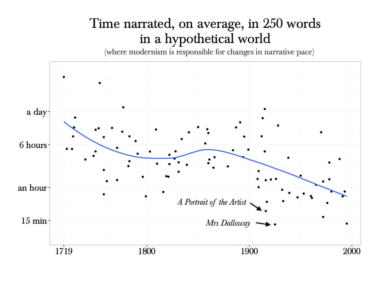
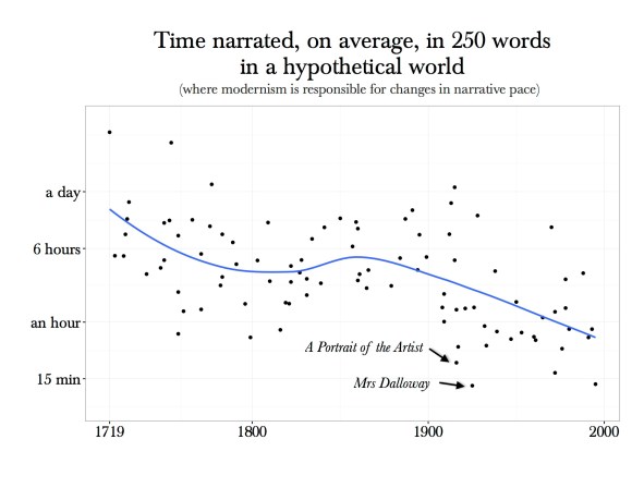


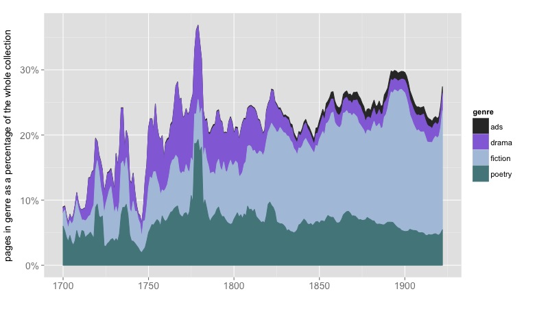
![Frequency of reference to "specific amounts" of money in 7,700 English-language works of fiction. Graphics from Wickham, ggplot2 [2].](https://tedunderwood.com/wp-content/uploads/2014/12/finalfreq.jpeg)