Categories
deep learning fiction

Using GPT-4 to measure the passage of time in fiction

Language models have been compared to parrots, but the bigger danger is that they turn people into parrots. A student who asks for “a paper about Middlemarch,” for instance, will get a pastiche loosely based on many things in the model’s training set. This may not count as plagiarism, but it won’t produce anything new.

But there are ways to use language models actively and creatively. We can select evidence to be analyzed, put it in a prompt, and specify the questions to be asked. Used this way, language models can create new knowledge that didn’t exist when they were trained. There are many ways to do this, and people may eventually get quite creative. But let’s start with a familiar task, so we can evaluate the results and decide whether language models really help. An obvious place to start is “content analysis”—a research method that analyzes hundreds or thousands of documents by posing questions about specific themes.

Below I work through a simple example of content analysis using the OpenAI API to measure the passage of time in fiction (see this GitHub repo for code). To spoil the suspense: I find that for this task, language models add something valuable, not just because they’re more accurate than older ways of doing this at scale but because they explain themselves better.

Why measure time in fiction?

Researchers already have several good ways to automate content analysis. Named entity extraction addresses certain kinds of questions. Topic modeling addresses others.

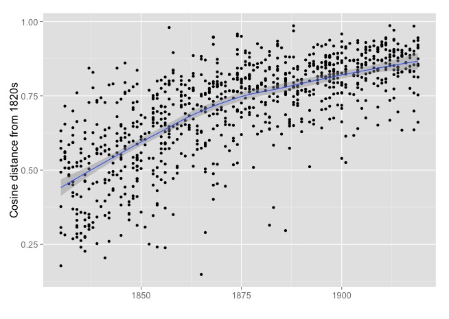
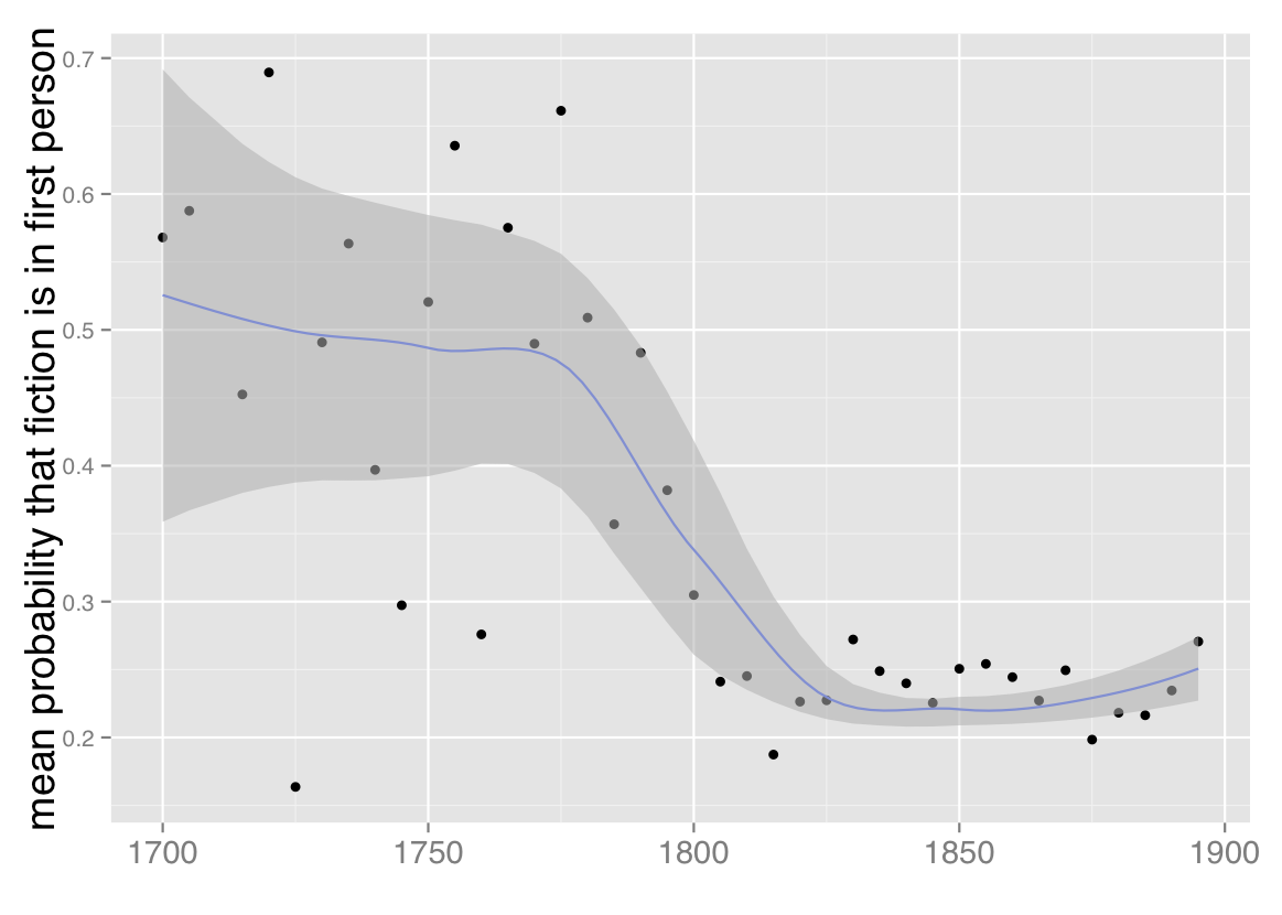
But there are also tricky questions that remain hard to answer by counting words. In 2017, for instance, I started to wonder how much time passes, on average, across a page of a novel. Literary-critical tradition suggested that there had been a pretty stable balance between “scene” (minute-by-minute description) and “summary” (which may cover weeks or years) until modernists started to leave out the summary and make every page breathlessly immediate [1]. But when I sat down with two graduate students (Sabrina Lee and Jessica Mercado) to manually characterize a thousand passages from fiction, we found instead a long trend. The average length of time represented in 250 words of fiction had been getting steadily shorter since the early eighteenth century. There was a trend toward immediacy, in other words, but modernism didn’t begin the trend [2].


The average length of time described in 250 words of narration. Y axis is logarithmic. The shaded ribbon represents a 95% confidence interval for the dashed curve, which is itself calculated by loess regression. From Underwood, “Why Literary Time is Measured in Minutes,” p. 352.

How well do bag of-words methods estimate time?

We decided to characterize passages manually because references to time in fiction can’t always be taken literally. If a character thinks (or says) “wow, it’s been thirty years but feels like yesterday,” you don’t want to conclude that thirty years have passed on the page. So word-counting seemed risky. Even as human readers we often found it hard to decide how much time was passing. But when a passage was read by two different people, our estimates agreed with each other well enough to conclude that “fictive time” was a meaningful construct, if not a precise one (r = .74 on log-transformed durations).

A year after we published our paper, Greg Yauney showed that word-counting methods can do an acceptable job of estimating time [3]. He trained a bag-of-words model on the passages we had labeled, and applied it to a new set of passages labeled by new readers. The model-predicted durations correlated with human estimates at r = .35. While this is much lower than inter-human agreement, the model was stable enough to precisely measure a trend (across thousands of books) that matched the trend we had sketched using laborious human reading of a hundred books.

From Yauney, Underwood, and Mimno, “Computational Prediction of Elapsed Narrative Time.”

Replicating this on our old data, I get a slightly higher correlation between models and readers (r = .49 on log-transformed durations), perhaps because the data I’m using was produced by readers who compared notes for several weeks to maximize agreement. But since this is still lower than .74, bag-of-words models are definitely less good at estimating time than human readers.

Can we train LLMs to estimate time?

To get a large language model to answer a question, you first need to make sure it understands the question. As Simon Willison helpfully explains, the way to train a chat model through the API is to demonstrate the interaction you want by providing a series of imagined exchanges between a “user” and an “assistant” [4]. These aren’t real replies from the assistant but ego ideals you’re providing to teach it how to behave.

Here’s the instruction I had the “user” give:

Read the following passage of fiction. Then do five things.
 
1: Briefly summarize the passage.
2: Reason step by step to decide how much time is described in the passage. If the passage doesn't include any explicit reference to time, you can guess how much time the events described would have taken. Even description can imply the passage of time by describing the earlier history of people or buildings. But characters' references to the past or future in spoken dialogue should not count as time that passed in the scene. Report the time using units of years, weeks, days, hours, or minutes. Do not say zero or N/A.
3: If you described a range of possible times in step 2 take the midpoint of the range. Then multiply to convert the units into minutes.
4: Report only the number of minutes elapsed, which should match the number in step 3. Do not reply N/A.
5: Given the amount of speculation required in step 2, describe your certainty about the estimate--either high, moderate, or low.
The passage follows: <omitting this to save space>

You’ll notice that I’m using chain-of-thought prompting, building slowly from summary to inference to an estimated number of minutes. You may also notice I tell the model twice “don’t reply N/A.” I found the model was pretty cautious about speculating and needed to be encouraged to make assumptions and guesses. But to be honest, it’s possible that the model was right to be cautious! Duration is hard to estimate in some cases, and maybe we humans should have allowed N/A responses when we did this.

Here’s an example of an ego-ideal reply I provided to teach the “assistant” how to respond. This was responding to a passage from The Big Sleep.

1: A detective wakes up 'the next morning,' looks out a window for an undefined time, drinks (and presumably needs to make) two cups of coffee, then shaves and showers and gets dressed before stepping out his front door and seeing a car.
2: Making coffee, showering, and getting dressed take at least an hour. There's some ambiguity about whether to count the implicit reference to yesterday (since this is 'the next morning') as time elapsed in the passage, but let's say no, since yesterday is not actually described. So, an hour to 90 minutes.
3: 1.25 hours have elapsed. Multiplying by 60 minutes an hour that's 75 minutes.
4: 75 minutes.
5: Low confidence, because of ambiguity about a reference to the previous day.

Using some code generously shared by Quinn Dombrowski, I gave the model four query-reply sequences like this, then asked it to characterize a new passage with the same instructions.

To assess performance on this simple task, I just extracted the minutes reported in step 4 and compared them to our human estimates from 2017. Other forms of content analysis might require the model to edit or mark up the text provided in the prompt. That’s doable, but I thought I would start with something simple.

I added step 5 (allowing the model to describe its own confidence) because in early experiments I found the model’s tendency to editorialize extremely valuable. The answers to step 5 were also fun to read as replies scrolled up the page, because my new sorcerer’s assistant complained volubly about the ambiguity of its task. (“30 minutes. Low confidence, as the passage is more focused on the poetic and symbolic aspects of the scene rather than providing a clear sense of time.”). In some cases it refused the task altogether and threw the question about confidence back in my face. (“N/A. High confidence that no specific amount of time is described.”) This capacity for backtalk is a feature not a bug: I learned a lot from it.

But after I adjusted my prompt to address the ambiguities the assistant correctly pointed out, complete refusal to answer the question was rare.

How well does GPT-4 estimate time?

I had the Turbo model code 483 passages. Its predictions correlated with human estimates at r = .59. I only asked GPT-4 to code 121 passages (because it’s more expensive to run than Turbo), and it achieved r = .68. This is not as good as inter-human agreement (.74), but it’s closer to human readers than to bag of words models (.35 – .49). And of course GPT-4 does the work more quickly than human readers. It took the three of us several months to generate this data, but my LLM experiment was run in a couple of days. Plus, given an API, large language models are easier to use than other forms of machine learning: the main challenge is to describe your question systematically. This is a method that could realistically be used by researchers with relatively little programming experience.

The total cost to my OpenAI account was $22. Of that amount, about $8 was testing the prompts and running on the (cheaper) Turbo API. The final run on GPT-4 cost $14; if I had completely replicated our work from 2017 on GPT-4 it would have cost $140. So a project like this will not bankrupt researchers. But reliance on OpenAI is still a bad idea in the long run. Universities should develop their own models and APIs, both for reasons of institutional autonomy/survival (!!😬!!) and so that researchers can inspect and tune the models.

However, one could exaggerate the problems of interpretability created by a closed model. Watching the model think out loud about each passage actually gave me a better sense of how results were produced than I could extract from my own records of human research in 2017. (See below for an example from GPT-4: human readers don’t usually document their thought process this verbosely.) Also, because human beings can’t erase their own memories, it’s not possible for us to “repeat the same question with slightly different language.” If I try that on myself, I’m going to remember what I thought before and probably think it again. But a model can wake up each moment with eternal sunshine of the spotless mind.

ABRIDGED PASSAGE FROM Jane Eyre: And signs, for aught we know, may be but the sympathies of Nature with man. When I was a little girl, only six years old, I one night heard Bessie Leaven say to Martha Abbot that she had been dreaming about a little child ... Of late I had often recalled this saying and this incident; for during the past week scarcely a night had gone over my couch that had not brought with it a dream of an infant, which I sometimes hushed in my arms, sometimes dandled on my knee, sometimes watched playing with daisies on a lawn, or again, dabbling its hands in running water. It was a wailing child this night, and a laughing one the next: now it nestled close to me, and now it ran from me; but whatever mood the apparition evinced, whatever aspect it wore, it failed not for seven successive nights to meet me the moment I entered the land of slumber.

ASSISTANT REPLIES. 1: The narrator recalls a saying about dreaming of children being a sign of trouble and remembers an incident from her childhood. She then describes her recent dreams of infants over the past week. 
2: The passage mentions the narrator's childhood memory, which happened when she was six years old, and the past week of dreams. The time elapsed in the passage is the week of dreams. 
3: 1 week has elapsed. At seven days a week that's 7 days. 24 hours in a day, so 168 hours. 60 minutes in an hour, so 10080 minutes. 
4: 10080 minutes. 
5: Moderate confidence, as the childhood memory is not counted as time passing in the scene.

What no model can do

While I think large language models will be tremendously useful assistants in content analysis, I don’t think we can dispense with multiple human readers. As David Bamman explains in a good Twitter thread, the core challenges of this work are “a. coming up with a new construct to measure, b. demonstrating that it can be measured, and c. showing that there’s value in doing so.” Intersubjective agreement between human beings is still the only way to know that we have addressed those questions.

That’s why I wouldn’t feel comfortable just making up my own definition of, say, “suspense,” teaching a model to measure it, and then running the model across a thousand books. The problem with that approach is not that LLMs have measurement error. (As we’ve seen in Greg Yauney’s paper, measurement methods with much more error can be productive.) The problem is that it isn’t clear what a single researcher’s construct means in the first place. To be confident that we’re measuring something called “suspense” we need to show that multiple people recognize it as suspense. And in spite of all the rhetorical personification in this blog post (which I trust you have understood rhetorically), a model is not a separate person. So a project of this kind still needs to start by getting several human beings to read systematically and compare notes, before the human codebook is translated into a prompt.

On the other hand, I do think language models will allow us to pose questions that are currently hard to pose at scale. Questions about plot and character, for instance, require reading a whole book while applying delicate decision criteria that may be hard to remember and keep stable across many books. Language models will help here not just because they’re fast, but because they can provide a relatively stable yardstick by which to measure slippery concepts, even at a modest scale of analysis.

This is a preliminary report on a very strange world. For me, the most surprising take-away from this experiment was not that deep learning is more accurate than statistical NLP, but that it may also be in some ways more interpretable. Because a language model has to think out loud, it tends to automatically document its own reasoning. This is useful even when (or especially when) the model doesn’t think you’ve defined the construct it’s supposed to measure clearly enough.

References

[1] Gérard Genette, Narrative Discourse: An Essay in Method, trans. Jane E. Lewin (Ithaca: Cornell Univ. Press, 1980), 97.

[2] Ted Underwood, “Why Literary Time is Measured in Minutes,” New Literary History 85.2 (2018) 351-65.

[3] Greg Yauney, Ted Underwood, and David Mimno, “Computational Prediction of Elapsed Narrative Time” (2019).

[4] Simon Willison, “A Simple Python Wrapper for the ChatGPT API” (2023).

Categories
character fiction

The instability of gender

Ted Underwood and David Bamman

1500-word abstract of a paper delivered Sat, Jan 9th, at MLA 2016, in a panel with Deidre Lynch and Andrew Piper. (An article based on this research, and further research with Sabrina Lee, will appear in Cultural Analytics in early 2018.)

helpfulBy visualizing course evaluations, Ben Schmidt has reminded us how subtly (and irrationally) descriptions of real people are shaped by gendered expectations. Men are praised for being funny, and condemned for being boring. Women are praised for being helpful, and condemned for being strict.

Fictional characters are never simply imagined people; they’re also aspects of novelistic form (Lynch 1998). But gendered patterns of description do appear in fiction, and it might be interesting to know how those patterns have changed. This also happens to be a problem where natural language processing can help us, since English pronouns have grammatical gender. (The gender of “me” is a trickier problem; for the purposes of this paper, we have regretfully set first-person narrators aside.)

We used BookNLP (a pipeline developed in Bamman et al. 2014a) to identify characters and the words connected to them. We applied it to 45,000 works of fiction distributed (unevenly) over the period 1780-1989. (The works themselves were partly drawn from HathiTrust and partly located at the Chicago Text Lab.) BookNLP does make errors (Vala et al., 2015), and any analysis on this scale will miss a great deal that is implied rather than said. But readers are so interested in character that it may be worth putting up with some gaps and uncertainties in order to glimpse broad historical patterns.

We asked, first, how strongly characterization is shaped by gender, and how that pressure waxed or waned across time. For instance, if you didn’t have names or pronouns, or tautological clues like “her Ladyship” and “her girlhood,” how easy would it be to infer a character’s (grammatical) gender from the apparently-genderless verbs, nouns, and adjectives associated with her?

One way to find out is to train a model to predict gender just from those implicit clues, testing it against the ground truth established by pronouns. When we do this, a long-term trend is perceptible: the linguistic differences between male and female characters get clearer to the middle of the nineteenth century, and then slowly get blurrier, through at least the 1980s.

Boxplots for 12 regularized logistic models in each decade; each model included 750 male and 750 female characters, randomly selected with the proviso that the median character size was always 51 words, and characters with less than 15 words were excluded.

It’s not a huge or dramatic shift, partly because gender is never easy to infer in the first place. (Since the model could get 50% of the characters right by guessing randomly, 74% is not eagle-eyed. Of course, the median character was only associated with 51 words, which is not a lot of evidence to go on.)

There are also questions about the data that make it difficult to be confident about details. We have sparse data before 1810, so we’re not certain yet that gender was really less clearly marked in the eighteenth century — although Virginia Woolf does tell us that “the sexes drew further and further apart” as the nineteenth century began (Woolf 1992: 219).

Also, after 1923, our dataset gets a little more American and a little better at excluding reprints, so the apparent acceleration of change from 1910 to 1930 might partly reflect changes in the corpus. In the final draft, we plan to check multiple corpora against each other. But we don’t have much doubt about the broad trend from 1840 to 1989. Over that century and a half, the boundary that separates “men” and “women” in fiction does seem to get blurrier and blurrier.

What were the tacit patterns that made it possible to predict a character’s gender in the first place, and how did they change? That’s a big question; there’s room here for several decades of discussion.

But some of the broadest patterns are easy to grasp. For each word, you can measure the difference between its frequency in descriptions of women and of men. (In the graphs below, words above zero are more common in descriptions of women.) Then you can sort the words to find ones where the difference between genders is large early in the period, and declines over time.

heartmindWhen you do that, you find a lot of words that describe subjective consciousness and emotion; most of them are attributed to women. “Passion” is an exception used more often for men; of course, in the early nineteenth century, it often means “lust.”

This evidence tends to support Nancy Armstrong’s contention in Desire and Domestic Fiction that subjectivity was to begin with “a female domain” in the novel (Armstrong 4), although it puts the peak of this phenomenon a little later than she suggests.

But in general, the gendering of subjectivity is a pattern that will be familiar to scholars of the novel. So, probably, is the tension between public and private space revealed here. Throughout the nineteenth century, it’s “her chamber” and “her room,” but “his country.” Around 1925, houses switch owners.

roominhouse

The convergence of all these lines on the right side of the graph helps explain why our models find gender harder and harder to predict: many of the words you might use to predict it are becoming less common (or becoming more evenly balanced between men and women — the graphs we’ve presented here don’t yet distinguish those two sorts of change.) On balance, that’s the prevailing trend. But there are also a few implicitly gendered forms of description that do increase. In particular, physical description becomes more important in fiction (Heuser and Le-Khac 2012).

From the Famous Artists' School course materials. "The male head is square and angular, with a strong jaw."
From the Famous Artists’ School course materials. “The male head is square and angular, with a strong jaw.”

And as writers spend more time describing their characters physically, some aspects of the body and dress also become more important as signifiers of gender. This isn’t a simple, monolithic process. There are parts of the body whose significance seems to peak at a certain date and then level off — like the masculine jaw, maybe peaking around 1950?

jawchest

Other signifiers of masculinity — like the chest, and incidentally pockets — continue to become more and more important. For women, the “eyes” and “face” peak very markedly around 1890. But hair has rarely been more gendered (or bigger) than it was in the 1980s.

eyeshairface

The measures we’re using here are simple, and deliberately conflate sheer frequency with gendered-ness in order to highlight words that have both attributes. We may use a wider range of interpretive strategies in the final article. But it’s clear already that gender has been unstable, not just because the implicit gendering of characterization became blurrier overall from 1840 to 1989 — but because the specific clues associated with gender have been rather volatile. In other words, gender is not at all the same thing in 1980 that it was in 1840.

There’s nothing very novel about the discovery that gender is fluid. But of course, we like to say everything is fluid: genres, roles, geographies. The advantage of a comparative method is that it lets us say specifically what we mean. Fluid compared to what? For instance, the increasing blurriness of gender boundaries is a kind of change we don’t see when we model the boundary between detective fiction and other genres: that boundary remains remarkably stable from 1841 to 1989. So we can say the linguistic signs of gender in characterization are more mutable than at least some genres.

We didn’t have to start with a complex data model to find this fluidity. Our initial representation of gender was a naive binary one, borrowed casually from English grammar. But we still ended up discovering that the things associated with those binary reference points have been in practice very changeable.

Other approaches are possible. The model Underwood has used to define genre (in a forthcoming piece) is messy and perspectival from the get-go, patched together from different sources of testimony. A project working with appropriate kinds of evidence could, similarly, build a perspectival dimension into definitions of gender from the very outset (for inspiration see Posner 2015 and Bamman et al. 2014b). But the point of research is also to discover things that weren’t hard-coded in the original plan. Even a perspectival model of genre may end up finding that different sources actually agree, for instance, about the boundaries of detective fiction. Conversely, even naively grammatical gender categories may start to bend and blur if they’re stretched across a two-century timeline.

Acknowledgements. This project was made possible by generous support from the NovelTM project, funded by the Social Sciences and Humanities Research Council. The authors would like to acknowledge work in progress at NovelTM as an influence on their thinking, including especially a forthcoming project by Matthew L. Jockers and Gabi Kirilloff. Our models of the twentieth century depend on collections located at the Chicago Text Lab, and supported by the University of Chicago Knowledge Lab. Eleanor Courtemanche suggested the connection to Woolf. BookNLP is available on github; work planned for this year at HathiTrust Research Center will make it possible for scholars to apply it to fiction even beyond the wall of copyright.

References:

Armstrong, Nancy. 1987. Desire and Domestic Fiction: A Political History of the Novel. New York: Oxford University Press.

Bamman, David, Ted Underwood, and Noah Smith. 2014a. “A Bayesian mixed-effects model of literary character.” ACL 2014. http://www.ark.cs.cmu.edu/literaryCharacter/

Bamman, David, Jacob Eisenstein, and Tyler Schnoebelen. 2014b. Gender Identity and Lexical Variation in Social Media. Journal of Sociolinguistics 18, 2 (2014).

Heuser, Ryan, and Long Le-Khac. 2012. “A Quantitative Literary History of 2,958 Nineteenth-Century British Novels: The Semantic Cohort Method.” Stanford Literary Lab Pamphlet Series. http://litlab.stanford.edu/pamphlets/ May 2012.

Lynch, Deidre. The Economy of Character: Novels, Market Culture, and the Business of Inner Meaning. Chicago: The University of Chicago Press, 1998.

Posner, Miriam. 2015. “What’s Next: The Radical, Unrealized Potential of Digital Humanities.” http://miriamposner.com/blog/whats-next-the-radical-unrealized-potential-of-digital-humanities/

Schmidt, Benjamin. 2015. “Gendered language in teaching reviews.” http://benschmidt.org/profGender/

Vala, Hardik, David Jurgens, Andrew Piper, and Derek Ruths. 2015. “Mr Bennet, his Coachman, and the Archibishop Walk into a Bar, but only One of them Gets Recognized.” CEMNLP. http://cs.stanford.edu/~jurgens/docs/vala-jurgens-piper-ruths_emnlp_2015.pdf

Woolf, Virginia. 1992. Orlando: A Biography, ed. Rachel Bowlby. Oxford: Oxford University Press.

Categories
historicism math methodology pace of historical change

Can we date revolutions in the history of literature and music?

Humanists know the subjects we study are complex. So on the rare occasions when we describe them with numbers at all, we tend to proceed cautiously. Maybe too cautiously. Distant readers have spent a lot of time, for instance, just convincing colleagues that it might be okay to use numbers for exploratory purposes.

But the pace of this conversation is not entirely up to us. Outsiders to our disciplines may rush in where we fear to tread, forcing us to confront questions we haven’t faced squarely.

For instance, can we use numbers to identify historical periods when music or literature changed especially rapidly or slowly? Humanists have often used qualitative methods to make that sort of argument. At least since the nineteenth century, our narratives have described periods of stasis separated by paradigm shifts and revolutionary ruptures. For scientists, this raises an obvious, tempting question: why not actually measure rates of change and specify the points on the timeline when ruptures happened?

The highest-profile recent example of this approach is an article in Royal Society Open Science titled “The evolution of popular music” (Mauch et al. 2015). The authors identify three moments of rapid change in US popular music between 1960 and 2010. Moreover, they rank those moments, and argue that the advent of rap caused popular music to change more rapidly than the British Invasion — a claim you may remember, because it got a lot of play in the popular press. Similar arguments have appeared about the pace of change in written expression — e.g, a recent article argues that 1917 was a turning point in political rhetoric (h/t Cameron Blevins).

When disciplinary outsiders make big historical claims, humanists may be tempted just to roll our eyes. But I don’t think this is a kind of intervention we can afford to ignore. Arguments about the pace of cultural change engage theoretical questions that are fundamental to our disciplines, and questions that genuinely fascinate the public. If scientists are posing these questions badly, we need to explain why. On the other hand, if outsiders are addressing important questions with new methods, we need to learn from them. Scholarship is not a struggle between disciplines where the winner is the discipline that repels foreign ideas with greatest determination.

I feel particularly obligated to think this through, because I’ve been arguing for a couple of years that quantitative methods tend to reveal gradual change rather than the sharply periodized plateaus we might like to discover in the past. But maybe I just haven’t been looking closely enough for discontinuities? Recent articles introduce new ways of locating and measuring them.

This blog post applies methods from “The evolution of popular music” to a domain I understand better — nineteenth-century literary history. I’m not making a historical argument yet, just trying to figure out how much weight these new methods could actually support. I hope readers will share their own opinions in the comments. So far I would say I’m skeptical about these methods — or at least skeptical that I know how to interpret them.

How scientists found musical revolutions.

Mauch et al. start by collecting thirty-second snippets of songs in the Billboard Hot 100 between 1960 and 2010. Then they topic-model the collection to identify recurring harmonic and timbral topics. To study historical change, they divide the fifty-year collection into two hundred quarter-year periods, and aggregate the topic frequencies for each quarter. They’re thus able to create a heat map of pairwise “distances” between all these quarter-year periods. This heat map becomes the foundation for the crucial next step in their argument — the calculation of “Foote novelty” that actually identifies revolutionary ruptures in music history.

Figure 5 from Mauch, et. al., “The evolution of popular music” (RSOS 2015).
The diagonal line from bottom left to top right of the heat map represents comparisons of each time segment to itself: that distance, obviously, should be zero. As you rise above that line, you’re comparing the same moment to quarters in its future; if you sink below, you’re comparing it to its past. Long periods where topic distributions remain roughly similar are visible in this heat map as yellowish squares. (In the center of those squares, you can wander a long way from the diagonal line without hitting much dissimilarity.) The places where squares are connected at the corners are moments of rapid change. (Intuitively, if you deviate to either side of the narrow bridge there, you quickly get into red areas. The temporal “window of similarity” is narrow.) Using an algorithm outlined by Jonathan Foote (2000), the authors translate this grid into a line plot where the dips represent musical “revolutions.”

Trying the same thing on the history of the novel.

Could we do the same thing for the history of fiction? The labor-intensive part would be coming up with a corpus. Nineteenth-century literary scholars don’t have a Billboard Hot 100. We could construct one, but before I spend months crafting a corpus to address this question, I’d like to know whether the question itself is meaningful. So this is a deliberately rough first pass. I’ve created a sample of roughly 1000 novels in a quick and dirty way by randomly selecting 50 male and 50 female authors from each decade 1820-1919 in HathiTrust. Each author is represented in the whole corpus only by a single volume. The corpus covers British and American authors; spelling is normalized to modern British practice. If I were writing an article on this topic I would want a larger dataset and I would definitely want to record things like each author’s year of birth and nationality. This is just a first pass.

Because this is a longer and sparser sample than Mauch et al. use, we’ll have to compare two-year periods instead of quarters of a year, giving us a coarser picture of change. It’s a simple matter to run a topic model (with 50 topics) and then plot a heat map based on cosine similarities between the topic distributions in each two-year period.

Heatmap and Foote novelty for 1000 novels, 1820-1919. Rises in the trend lines correspond to increased Foote novelty.
Voila! The dark and light patterns are not quite as clear here as they are in “The evolution of popular music.” But there are certainly some squarish areas of similarity connected at the corners. If we use Foote novelty to interpret this graph, we’ll have one major revolution in fiction around 1848, and a minor one around 1890. (I’ve flipped the axis so peaks, rather than dips, represent rapid change.) Between these peaks, presumably, lies a valley of Victorian stasis.

Is any of that true? How would we know? If we just ask whether this story fits our existing preconceptions, I guess we could make it fit reasonably well. As Eleanor Courtemanche pointed out when I discussed this with her, the end of the 1840s is often understood as a moment of transition to realism in British fiction, and the 1890s mark the demise of the three-volume novel. But it’s always easy to assimilate new evidence to our preconceptions. Before we rush to do it, let’s ask whether the quantitative part of this argument has given us any reason at all to believe that the development of English-language fiction really accelerated in the 1840s.

I want to pose four skeptical questions, covering the spectrum from fiddly quantitative details to broad theoretical doubts. I’ll start with the fiddliest part.

1) Is this method robust to different ways of measuring the “distance” between texts?

The short answer is “yes.” The heat maps plotted above are calculated on a topic model, after removing stopwords, but I get very similar results if I compare texts directly, without a topic model, using a range of different distance metrics. Mauch et al. actually apply PCA as well as a topic model; that doesn’t seem to make much difference. The “moments of revolution” stay roughly in the same place.

2) How crucial is the “Foote novelty” piece of the method?

Very crucial, and this is where I think we should start to be skeptical. Mauch et al. are identifying moments of transition using a method that Jonathan Foote developed to segment audio files. The algorithm is designed to find moments of transition, even if those moments are quite subtle. It achieves this by making comparisons — not just between the immediately previous and subsequent moments in a stream of observations — but between all segments of the timeline.

It’s a clever and sensitive method. But there are other, more intuitive ways of thinking about change. For instance, we could take the first ten years of the dataset as a baseline and directly compare the topic distributions in each subsequent novel back to the average distribution in 1820-1829. Here’s the pattern we see if we do that:

byyearThat looks an awful lot like a steady trend; the trend may gradually flatten out (either because change really slows down or, more likely, because cosine distances are bounded at 1.0) but significant spurts of revolutionary novelty are in any case quite difficult to see here.

That made me wonder about the statistical significance of “Foote novelty,” and I’m not satisfied that we know how to assess it. One way to test the statistical significance of a pattern is to randomly permute your data and see how often patterns of the same magnitude turn up. So I repeatedly scrambled the two-year periods I had been comparing, constructed a heat matrix by comparing them pairwise, and calculated Foote novelty.

A heatmap produced by randomly scrambling the fifty two-year periods in the corpus. The “dates” on the timeline are now meaningless.
When I do this I almost always find Foote novelties that are as large as the ones we were calling “revolutions” in the earlier graph.

The authors of “The evolution of popular music” also tested significance with a permutation test. They report high levels of significance (p < 0.01) and large effect sizes (they say music changes four to six times faster at the peak of a revolution than at the bottom of a trough). Moreover, they have generously made their data available, in a very full and clearly-organized csv. But when I run my permutation test on their data, I run into the same problem — I keep discovering random Foote novelties that seem as large as the ones in the real data.

It’s possible that I’m making some error, or that we're testing significance differently. I'm permuting the underlying data, which always gives me a matrix that has the checkerboardy look you see above. The symmetrical logic of pairwise comparison still guarantees that random streaks organize themselves in a squarish way, so there are still “pinch points” in the matrix that create high Foote novelties. But the article reports that significance was calculated “by random permutation of the distance matrix.” If I actually scramble the rows or columns of the distance matrix itself I get a completely random pattern that does give me very low Foote novelty scores. But I would never get a pattern like that by calculating pairwise distances in a real dataset, so I haven’t been able to convince myself that it’s an appropriate test.

3) How do we know that all forms of change should carry equal cultural weight?

Now we reach some questions that will make humanists feel more at home. The basic assumption we’re making in the discussion above is that all the features of an expressive medium bear historical significance. If writers replace “love” with “spleen,” or replace “cannot” with “can’t,” it may be more or less equal where this method is concerned. It all potentially counts as change.

This is not to say that all verbal substitutions will carry exactly equal weight. The weight assigned to words can vary a great deal depending on how exactly you measure the distance between texts; topic models, for instance, will tend to treat synonyms as equivalent. But — broadly speaking — things like contractions can still potentially count as literary change, just as instrumentation and timbre count as musical change in “The evolution of popular music.”

At this point a lot of humanists will heave a relieved sigh and say “Well! We know that cultural change doesn’t depend on that kind of merely verbal difference between texts, so I can stop worrying about this whole question.”

Not so fast! I doubt that we know half as much as we think we know about this, and I particularly doubt that we have good reasons to ignore all the kinds of change we’re currently ignoring. Paying attention to merely verbal differences is revealing some massive changes in fiction that previously slipped through our net — like the steady displacement of abstract social judgment by concrete description outlined by Heuser and Le-Khac in LitLab pamphlet #4.

For me, the bottom line is that we know very little about the kinds of change that should, or shouldn’t, count in cultural history. “The evolution of popular music” may move too rapidly to assume that every variation of a waveform bears roughly equal historical significance. But in our daily practice, literary historians rely on a set of assumptions that are much narrower and just as arbitrary. An interesting debate could take place about these questions, once humanists realize what’s at stake, but it’s going to be a thorny debate, and it may not be the only way forward, because …

4) Instead of discussing change in the abstract, we might get further by specifying the particular kinds of change we care about.

Our systems of cultural periodization tend to imply that lots of different aspects of writing (form and style and theme) all change at the same time — when (say) “aestheticism” is replaced by “modernism.” That underlying theory justifies the quest for generalized cultural growth spurts in “The evolution of popular music.”

But we don’t actually have to think about change so generally. We could specify particular social questions that interest us, and measure change relative to those questions.

The advantage of this approach is that you no longer have to start with arbitrary assumptions about the kind of “distance” that counts. Instead you could use social evidence to train a predictive model. Insofar as that model predicts the variables you care about, you know that it’s capturing the specific kind of change that matters for your question.

Jordan Sellers and I took this approach in a working paper we released last spring, modeling the boundary between volumes of poetry that were reviewed in prominent venues, and those that remained obscure. We found that the stylistic signals of poetic prestige remained relatively stable across time, but we also found that they did move, gradually, in a coherent direction. What we didn’t do, in that article, is try to measure the pace of change very precisely. But conceivably you could, using Foote novelty or some other method. Instead of creating a heatmap that represents pairwise distances between texts, you could create a grid where models trained to recognize a social boundary in particular decades make predictions about the same boundary in other decades. If gender ideologies or definitions of poetic prestige do change rapidly in a particular decade, it would show up in the grid, because models trained to predict authorial gender or poetic prominence before that point would become much worse at predicting it afterward.

Conclusion

I haven’t come to any firm conclusion about “The evolution of popular music.” It’s a bold article that proposes and tests important claims; I’ve learned a lot from trying the same thing on literary history. I don’t think I proved that there aren’t any revolutionary growth spurts in the history of the novel. It’s possible (my gut says, even likely) that something does happen around 1848 and around 1890. But I wasn’t able to show that there’s a statistically significant acceleration of change at those moments. More importantly, I haven’t yet been able to convince myself that I know how to measure significance and effect size for Foote novelty at all; so far my attempts to do that produce results that seem different from the results in a paper written by four authors who have more scientific training than I do, so there’s a very good chance that I’m misunderstanding something.

I would welcome comments, because there are a lot of open questions here. The broader task of measuring the pace of cultural change is the kind of genuinely puzzling problem that I hope we’ll be discussing at more length in the IPAM Cultural Analytics workshop next spring at UCLA.

Postscript Oct 5: More will be coming in a day or two. The suggestions I got from comments (below) have helped me think the quantitative part of this through, and I’m working up an iPython notebook that will run reliable tests of significance and effect size for the music data in Mauch et al. as well as a larger corpus of novels. I have become convinced that significance tests on Foote novelty are not a good way to identify moments of rapid change. The basic problem with that approach is that sequential datasets will always have higher Foote novelties than permuted (non-sequential) datasets, if you make the “window” wide enough — even if the pace of change remains constant. Instead, borrowing an idea from Hoyt Long and Richard So, I’m going to use a Chow test to see whether rates of change vary.

Postscript Oct 8: Actually it could be a while before I have more to say about this, because the quantitative part of the problem turns out to be hard. Rates of change definitely vary. Whether they vary significantly, may be a tricky question.

References:

Jonathan Foote. Automatic audio segmentation using a measure of audio novelty. In Proceedings of IEEE International Conference on Multimedia and Expo, vol. I, pp. 452-455, 2000.

Matthias Mauch, Robert M. MacCallum, Mark Levy, Armand M. Leroi. The evolution of popular music. Royal Society Open Science. May 6, 2015.

Categories
18c 19c fiction point of view representativeness

Genre, gender, and point of view.

A paper for the IEEE “big humanities” workshop, written in collaboration with Michael L. Black, Loretta Auvil, and Boris Capitanu, is available on arXiv now as a preprint.

The Institute of Electrical and Electronics Engineers is an odd venue for literary history, and our paper ends up touching so many disciplinary bases that it may be distracting.* So I thought I’d pull out four issues of interest to humanists and discuss them briefly here; I’m also taking the occasion to add a little information about gender that we uncovered too late to include in the paper itself.

1) The overall point about genre. Our title, “Mapping Mutable Genres in Structurally Complex Volumes,” may sound like the sort of impossible task heroines are assigned in fairy tales. But the paper argues that the blurry mutability of genres is actually a strong argument for a digital approach to their history. If we could start from some consensus list of categories, it would be easy to crowdsource the history of genre: we’d each take a list of definitions and fan out through the archive. But centuries of debate haven’t yet produced stable definitions of genre. In that context, the advantage of algorithmic mapping is that it can be comprehensive and provisional at the same time. If you change your mind about underlying categories, you can just choose a different set of training examples and hit “run” again. In fact we may never need to reach a consensus about definitions in order to have an interesting conversation about the macroscopic history of genre.

2) A workset of 32,209 volumes of English-language fiction. On the other hand, certain broad categories aren’t going to be terribly controversial. We can probably agree about volumes — and eventually specific page ranges — that contain (for instance) prose fiction and nonfiction, narrative and lyric poetry, and drama in verse, or prose, or some mixture of the two. (Not to mention interesting genres like “publishers’ ads at the back of the volume.”) As a first pass at this problem, we extract a workset of 32,209 volumes containing prose fiction from a collection of 469,200 eighteenth- and nineteenth-century volumes in HathiTrust Digital Library. The metadata for this workset is publicly available from Illinois’ institutional repository. More substantial page-level worksets will soon be produced and archived at HathiTrust Research Center.

3) The declining prevalence of first-person narration. Once we’ve identified this fiction workset, we switch gears to consider point of view — frankly, because it’s a temptingly easy problem with clear literary significance. Though the fiction workset we’re using is defined more narrowly than it was last February, we confirm the result I glimpsed at that point, which is that the prevalence of first-person point of view declines significantly toward the end of the eighteenth century and then remains largely stable for the nineteenth.

Mean probability that fiction is written in first person, 1700-1899. Based on a corpus of 32,209 volumes of fiction extracted from HathiTrust Digital Library. Points are mean probabilities for five-year spans of time; a trend line with standard errors has been plotted with loess smoothing.

We can also confirm that result in a way I’m finding increasingly useful, which is to test it in a collection of a completely different sort. The HathiTrust collection includes reprints, which means that popular works have more weight in the collection than a novel printed only once. It also means that many volumes carry a date much later than their first date of publication. In some ways this gives a more accurate picture of print culture (an approximation to “what everyone read,” to borrow Scott Weingart’s phrase), but one could also argue for a different kind of representativeness, where each volume would be included only once, in a record dated to its first publication (an attempt to represent “what everyone wrote”).

Mean probability that fiction is written in first person, 1700-1899. Based on a corpus of 774 volumes of fiction selected by multiple hands from multiple sources. Plotted in 20-year bins because n is small here. Works are weighted by the number of words they contain.
Mean probability that fiction is written in first person, 1700-1899. Based on a corpus of 774 volumes of fiction selected by multiple hands from multiple sources. Plotted in 20-year bins because n is smaller here. Works are weighted by the number of words they contain.

Fortunately, Jordan Sellers and I produced a collection like that a few years ago, and we can run the same point-of-view classifier on this very different set of 774 fiction volumes (metadata available), selected by multiple hands from multiple sources (including TCP-ECCO, the Brown Women Writers Project, and the Internet Archive). Doing that reveals broadly the same trend line we saw in the HathiTrust collection. No collection can be absolutely representative (for one thing, because we don’t agree on what we ought to be representing). But discovering parallel results in collections that were constructed very differently does give me some confidence that we’re looking at a real trend.

4. Gender and point of view. In the process of classifying works of fiction, we stumbled on interesting thematic patterns associated with point of view. Features associated with first-person perspective include first-person pronouns, obviously, but also number words and words associated with sea travel. Some of this association may be explained by the surprising persistence of a particular two-century-long genre, the Robinsonade. A castaway premise obviously encourages first-person narration, but the colonial impulse in the Robinsonade also seems to have encouraged acquisitive enumeration of the objects (goats, barrels, guns, slaves) its European narrators find on ostensibly deserted islands. Thus all the number words. (But this association of first-person perspective with colonial settings and acquisitive enumeration may well extend beyond the boundaries of the Robinsonade to other genres of adventure fiction.)

Third-person perspective, on the other hand, is durably associated with words for domestic relationships (husband, lover, marriage). We’re still trying to understand these associations; they could be consequences of a preference for third-person perspective in, say, courtship fiction. But third-person pronouns correlate particularly strongly with words for feminine roles (girl, daughter, woman) — which suggests that there might also be a more specifically gendered dimension to this question.

Since transmitting our paper to the IEEE I’ve had a chance to investigate this hypothesis in the smaller of the two collections we used for that paper — 774 works of fiction between 1700 and 1899: 521 by men, 249 by women, and four not characterized by gender. (Mike Black and Jordan Sellers recorded this gender data by hand.) In this collection, it does appear that male writers choose first-person perspective significantly more than women do. The gender gap persists across the whole timespan, although it might be fading toward the end of the nineteenth century.

Proportion of works of fiction by men and women in first person. Based on the same set of 774 volumes described above. (This figure counts strictly by the number of works rather than weighting works by the number of words they contain.)

Over the whole timespan, women use first person in roughly 23% of their works, and men use it in roughly 35% of their works.** That’s not a huge difference, but in relative terms it’s substantial. (Men are using first person 52% more than women). The Bayesian mafia have made me wary of p-values, but if you still care: a chi-squared test on the 2×2 contingency table of gender and point of view gives p < 0.001. (Attentive readers may already be wondering whether the decline of first person might be partly explained by an increase in the proportion of women writers. But actually, in this collection, works by women have a distribution that skews slightly earlier than that of works by men.)

These are very preliminary results. 774 volumes is a small set when you could test 32,209. At the recent HTRC Uncamp, Stacy Kowalczyk described a method for gender identification in the larger HathiTrust corpus, which we will be eager to borrow once it’s published. Also, the mere presence of an association between gender and point of view doesn’t answer any of the questions literary critics will really want to pose about this phenomenon — like, why is point of view associated with gender? Is this actually a direct consequence of gender, or is it an indirect consequence of some other variable like genre? Does this gendering of narrative perspective really fade toward the end of the nineteenth century? I don’t pretend to have answered any of those questions, all I’m doing here is flagging the existence of an interesting open question that will deserve further inquiry.

— — — — —

*Other papers for the panel are beginning to appear online. Here’s “Infectious Texts: Modeling Text Reuse in Nineteenth-Century Newspapers,” by David A. Smith, Ryan Cordell, and Elizabeth Maddock Dillon.

** We don’t actually represent point of view as a binary choice between first person or third person; the classifier reports probabilities as a continuous range between 0 and 1. But for purposes of this blog post I’ve simplified by dividing the works into two sets at the 0.5 mark. On this point, and for many other details of quantitative methodology, you’ll want to consult the paper itself.