Month: February 2011

Until recently, I’ve been limited to working with tools provided by other people. But in the last month or so I realized that it’s easier than it used to be to build these things yourself, so I gave myself a crash course in MySQL and R, with a bit of guidance provided by Ben Schmidt, whose blog Sapping Attention has been a source of many good ideas. I should also credit Matt Jockers and Ryan Heuser at the Stanford Literary Lab, who are doing fabulous work on several different topics; I’m learning more from their example than I can say here, since I don’t want to describe their research in excessive detail.

I’ve now been able to download Google’s 1gram English corpus between 1700 and 1899, and have normalized it to make it more useful for exploring the 18th and 19th centuries. In particular, I normalized case and developed a way to partly correct for the common OCR errors that otherwise make the Google corpus useless in the eighteenth century: especially the substitutions s->f and ss->fl.

Having done that, I built a couple of modules that mine the dataset for patterns. Last December, I was intrigued to discover that words with close semantic relationships tend to track each other closely (using simple sensory examples like the names of colors and oppositions like hot/cold). I suspected that this pattern might extend to more abstract concepts as well, but it’s difficult to explore that hypothesis if you have to test possible instances one by one. The correlation-seeking module has made it possible to explore it more rapidly, and has also put some numbers on what was before a purely visual sense of “fittedness.”

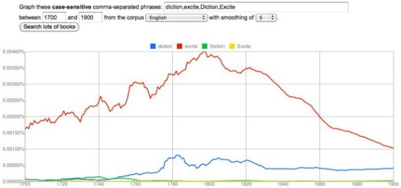
For instance, consider “diction.” It turns out that the closest correlate to “diction” in the period 1700-1899 is “versification,” which has a Pearson correlation coefficient of 0.87. (If this graph doesn’t seem to match the Google version, remember that the ngram viewer is useless in the 18c until you correct for case and long s.)

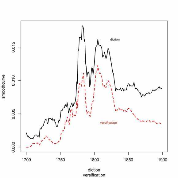
The other words that correlate most closely with “diction” are all similarly drawn from the discourse of poetic criticism. “Poem” and “stanzas” have a coefficient of 0.82; “poetical” is 0.81. It’s a bit surprising that correlation of yearly frequencies should produce such close thematic connections. Obviously, a given subject category will be overrepresented in certain years, and underrepresented in others, so thematically related words will tend to vary together. But in a corpus as large and diverse as Google’s, one might have expected that subtle variation to be swamped by other signals. In practice it isn’t.

I’ve also built a module that looks for words that are overrepresented in a given period relative to the rest of 1700-1899. The measures of overrepresentation I’m using are a bit idiosyncratic. I’m simply comparing the mean frequency inside the period to the mean frequency outside it. I take the natural log of the absolute difference between those means, and multiply it by the ratio (frequency in the period/frequency outside it). For the moment, that formula seems to be working; I’ll try other methods (log-likelihood, etc.) later on.

Once I find a list of, say, fifty words that are overrepresented in a period, I can generate a correlation matrix based on their correlations with each other, and then do hierarchical clustering on that matrix to reveal which words track each other most closely. In effect, I create a broad list of “trending topics” in a particular period, and then use a more precise sort of curve-matching to define the relationships between those trends.

One might imagine that matching words on the basis of change-across-time would be a blunt instrument compared to a more intimate approach based on collocation in the same sentences, or at least co-occurrence in the same volumes. And for many purposes that will be true. But I’ve found that my experiments with smaller-scale co-occurrence (e.g. in MONK) often lead me into tautological dead ends. I’ll discover, e.g., that historical novels share the kind of vocabulary I sort of knew historical novels were likely to share. Relying on yearly frequency data makes it easier to avoid those dead ends, because they have the potential to turn up patterns that aren’t based purely on a single familiar genre or subject category. They may be a blunt instrument, but through their very bluntness they allow us to back up to a vantage point where it’s possible to survey phenomena that are historical rather than purely semantic.

I’ve included an example below. The clusters that emerge here are based on a kind of semantic connection, but often it’s a connection that only makes sense in the context of the period. For instance, “nitrous” and “inflammable” may seem a strange pairing, unless you know that the recently-discovered gas hydrogen was called “inflammable air,” and that chemists were breathing nitrous oxide, aka laughing gas. “Sir” and “de” may seem a strange pairing, unless you reflect that “de” is a French particle of nobility analogous to “sir,” and so on. But I also find that I’m discovering a lot here I didn’t previously know. For instance, I probably should have guessed that Petrarch was a big deal in this period, since there was a sonnet revival — but that’s not something I actually knew, and it took me a while to figure out why Petrarch was coming up. I still don’t know why he’s connected to the dramatist Charles Macklin.

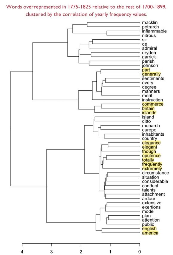
There are lots of other fun pairings in there, especially britain/commerce/islands and the group of flashy hyperbolic adverbs totally/frequently/extremely connected to elegance/opulence. I’m not sure that I would claim a graph like this has much evidentiary value; clustering algorithms are sensitive to slight shifts in initial conditions, so a different list of words might produce different groupings. But I’m also not sure that evidentiary value needs to be our goal. Lately I’ve been inclined to argue that the real utility of text mining may be as a heuristic that helps us discover puzzling questions. I certainly feel that a graph like this helps me identify topics (and more subtly, kinds of periodized diction) that I didn’t recognize before, and that deserve further exploration. [UPDATE 4/20/2011: Back in February I was doing this clustering with yearly frequency data, and Pearson’s correlation, which worked surprisingly well. But I’m now fairly certain that it’s better to do it with co-occurrence data, and a vector space model. See this more recent post.]

It’s only in the last few months that I’ve come to understand how complex search engines actually are. Part of the logic of their success has been to hide the underlying complexity from users. We don’t have to understand how a search engine assigns different statistical weights to different terms; we just keep adding terms until we find what we want. The differences between algorithms (which range widely in complexity, and are based on different assumptions about the relationship between words and documents) never cross our minds.

I’m pretty sure search engines have transformed literary scholarship. There was a time (I can dimly recall) when it was difficult to find new primary sources. You had to browse through a lot of bibliographies looking for an occasional lead. I can also recall the thrill I felt, at some point in the 90s, when I realized that full-text searches in a Chadwyck-Healey database could rapidly produce a much larger number of leads — things relevant to my topic, that no one else seemed to have read. Of course, I wasn’t the only one realizing this. I suspect the wave of challenges to canonical “Romanticism” in the 90s had a lot to do with the fact that Romanticists all realized, around the same time, that we had been looking at the tip of an iceberg.

One could debate whether search engines have exerted, on balance, a positive or negative influence on scholarship. If the old paucity of sources tempted critics to endlessly chew over a small and unrepresentative group of authors, the new abundance may tempt us to treat all works as more or less equivalent — when perhaps they don’t all provide the same kinds of evidence. But no one blames search engines themselves for this, because search isn’t an evidentiary process. It doesn’t claim to prove a thesis. It’s just a heuristic: a technique that helps you find a lead, or get a better grip on a problem, and thus abbreviates the quest for a thesis.

The lesson I would take away from this story is that it’s much easier to transform a discipline when you present a new technique as a heuristic than when you present it as evidence. Of course, common sense tells us that the reverse is true. Heuristics tend to be unimpressive. They’re often quite simple. In fact, that’s the whole point: heuristics abbreviate. They also “don’t really prove anything.” I’m reminded of the chorus of complaints that greeted the Google ngram viewer when it first came out, to the effect that “no one knows what these graphs are supposed to prove.” Perhaps they don’t prove anything. But I find that in practice they’re already guiding my research, by doing a kind of temporal orienteering for me. I might have guessed that “man of fashion” was a buzzword in the late eighteenth century, but I didn’t know that “diction” and “excite” were as well.

What does a miscellaneous collection of facts about different buzzwords prove? Nothing. But my point is that if you actually want to transform a discipline, sometimes it’s a good idea to prove nothing. Give people a new heuristic, and let them decide what to prove. The discipline will be transformed, and it’s quite possible that no one will even realize how it happened.

POSTSCRIPT, May 1, 2011: For a slightly different perspective on this issue, see Ben Schmidt’s distinction between “assisted reading” and “text mining.” My own thinking about this issue was originally shaped by Schmidt’s observations, but on re-reading his post I realize that we’re putting the emphasis in slightly different places. He suggests that digital tools will be most appealing to humanists if they resemble, or facilitate, familiar kinds of textual encounter. While I don’t disagree, I would like to imagine that humanists will turn out in the end to be a little more flexible: I’m emphasizing the “heuristic” nature of both search engines and the ngram viewer in order to suggest that the key to the success of both lies in the way they empower the user. But — as the word “tricked” in the title is meant to imply — empowerment isn’t the same thing as self-determination. To achieve that, we need to reflect self-consciously on the heuristics we use. Which means that we need to realize we’re already doing text mining, and consider building more appropriate tools.

This post was originally titled “Why Search Was the Killer App in Text-Mining.”