Category: discovery strategies

“Plot arcs” in the novel.

Ben Schmidt has developed a fascinating way of visualizing “plot arcs” in television series. I’ve been trying to understand how it works, with help from several people on Twitter, and also trying to see if it can reveal anything interesting about novels.

If you haven’t read Ben’s blog post, I recommend exploring it now, because I’m going to skim lightly over some of the details of his method.

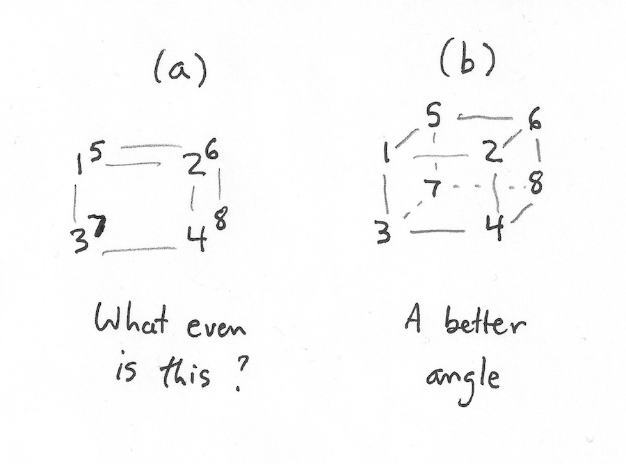
At its core, the technique is not complicated. It hinges on a transformation called principal component analysis (PCA), which allows researchers to map high-dimensional data onto a two-dimensional space, while keeping individual data points as far apart as possible. You can think of PCA as a technique that gives you a “good viewing angle” for flattening out a complex object. For instance, if you’ve got eight points at the corners of a cube, you could represent them as seen in (a), but (b) might be more legible because it spreads the points out more. It does that by squashing several different physical dimensions (length and breadth) into the x axis on the page.

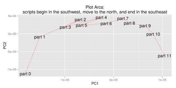
Ben uses this technique to reveal the structural relationship between different parts of a plot. As I understand it, he divides television scripts into six segments of equal length, and trains a topic model on all the segments. If you produce, say, 100 topics, each segment of each show is now characterized as a point in 100-dimensional space, where each dimension measures the prominence of one particular topic.

He takes the first sixth of every show and averages them to produce a single point that represents the average topic distribution for the first-sixth of all shows. After doing that for all six segments, he has six data points that represent typical segments of narrative time. Then he uses PCA to find an abstract space where those points are well separated. When he does this, he gets an arc-like structure that tends to preserve the original narrative sequence of the segments (although the algorithm isn’t directly informed about sequence). In his most detailed visualization, he even takes this down to twelfths.

Benjamin Schmidt's initial visualization of "plot arcs," December 16, 2014. — Benjamin Schmidt’s initial visualization of “plot arcs,” December 16, 2014.

But what does this mean?
From the beginning, Ben has been pretty careful to stress that he sees the parabolic shape of this pattern as an artifact of PCA. (“I should emphasize that it’s hard to imagine any other shape coming out of the PCA algorithm with the inputs I put in.”) David Bamman confirms this, showing that PCA will turn many kinds of sequential data, even random walks, into an arc. The algorithm is also good at inferring sequence: if point 1 influences point 2, and point 2 influences point 3, etc., PCA will tend to preserve their sequential relationship in the projection. (It does this even if you take 1000 different random walks and add them up to produce a composite walk.) So if we believe that the topic distribution in each segment of each story is strongly related to the topic distributions on either side, we would expect PCA to organize the composite segments of all stories in a sequential arc.

That’s sort of cool, but also suggests that the structure we’re seeing is not unique to “plots.” On the other hand, it’s worth noting that the technique does work better on fiction (and television scripts) than on nonfiction. Or, rather, it shows us something different when you apply it to nonfiction.

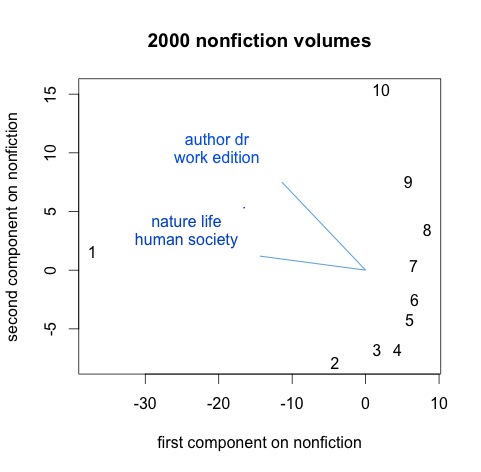
Here I’ve divided 2000 volumes of nineteenth-century nonfiction into ten parts, trained 200 topics on all 20,000 segments, and then created composite data points that represent the first “tenth,” second “tenth,” and so on, for all the volumes. PCA is still, somewhat remarkably, able to organize these points in the right sequence, but you have to squint a little to call this an arc. The graph is more clearly dominated by a contrast between introductions and body text. I’ve plotted two of the most important organizing topics as vectors; they include a lot of high-level abstractions and metadiscourse, whereas most of the topics in this nonfiction model are as specific as “birds eggs young wings” (and have a much smaller influence on this graph).

It’s important to note that I’m using the page-level metadata I recently described to select nonfiction here, which makes an effort to screen out paratext. (Otherwise we would probably be seeing topics like “table contents” and “index due date”!)

So where does this leave us? I think Lynn Cherny is right to say that with this technique, deviations from an arc are more significant than the arc itself. The slightly arc-like sequence on the right-hand side of the nonfiction graph isn’t telling us much about deep structures organizing nonfiction; it’s telling us mainly that there are continuities in text. But the “1” way over on the left-hand side is revealing a large structural fact: works of nonfiction have prefaces and introductions that can be very different from the rest of the text. Similarly, one of the most interesting aspects of Ben’s post involves the structural differences he finds toward the end between television genres (the difference between beginning and end seems more important for comedies, whereas science fiction is more organized by a contrast between central action and frame). Not a bad result for a historian to generate in his spare time.

Ten points that represent composite "tenths" of 1.981 works of fiction, topic-modeled and projected by PCA. Multivolume works have been joined. — Ten points that represent composite “tenths” of 1.981 works of fiction, topic-modeled and projected by PCA. Multivolume works have been joined.

Also, when I say differences are interesting, I don’t mean that the composite arc Ben saw by averaging all genres was meaningless. The fact that PCA will organize ten segments of 2000 novels into a parabola is not surprising. It would do that even with a random sequence. But in practice we’re not looking at random sequences, so PCA organizes points into a parabola by drawing on actual linguistic gradients that organize narrative time. As Ben has shown in a follow-up post, PCA is able to explain the patterns in television scripts better than it can explain random sequences.

In other words, the differences we’re seeing between beginnings, middles, and ends are real differences. And it’s interesting to see what those differences are. The x and y axes in a PCA projection don’t have simple meanings, because we’ve squashed multiple dimensions into two. But we can understand the space a little better by mapping the influence exerted by different topics.

Vectors that play an especially strong role in organizing the PCA projection of 1,981 nineteenth-century novels.

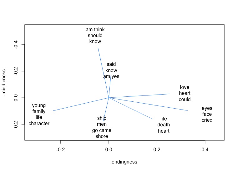
In this visualization, for instance, topics associated with dialogue (“said am know yes”) tend to move a point up the y axis. They’re more common in the middle of a narrative.

It might also be interesting to compare the way narratives from different authors or genres project into this space.

Each author here is represented by a composite set of ten segments of narrative time, produced by averaging her works. They are projected into a space defined by the average “tenths” of all works in the dataset.

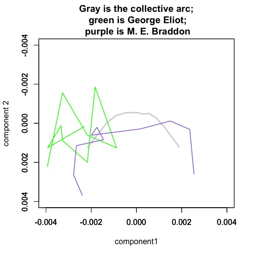
Mary Elizabeth Braddon is a sensation novelist, and her works are strongly organized by a structure that resembles the majority of other novels in the nineteenth century (or is perhaps even more distinct than usual). A book like Lady Audley’s Secret begins with a stage-setting description of domestic space and family relationships. The middle of the book is characterized by dialogue. The tone of the diction becomes progressively more sentimental* until, in the conclusion, we back away from dialogue again to summary (but a summary that is very different from the introduction in tone).

By contrast, the novels of George Eliot are… um, perhaps it would be safest to say “not as well characterized by this model of narrative sequence.” You might be tempted to look at that tangle of lines and infer some kind of cyclic structure, but it would be a bit like reading tea leaves. I know George Eliot’s novels are interesting, but I doubt that squiggle tells me why. (It’s important to remember, for instance, that Eliot’s narrative time looks more orderly and arc-like when projected into a space defined by her own writing.)

Supervised and unsupervised models
In short, I think the method Ben has developed is interesting and worth further exploration, but I also think there are real interpretive challenges here. And the interpretive challenges are not general problems that would arise with any quantitative method: they’re specific to a quirk of this one, which is that it’s poised delicately between strategies of “supervised” and “unsupervised” modeling.

Actually, I’m not sure it’s technically accurate to call PCA a model at all; it’s almost a descriptive statistic (like the mean or standard deviation of a dataset). But the attraction of the technique is a bit like the attraction of unsupervised modeling: you turn it loose on the data and it spontaneously reveals patterns.

There’s nothing at all wrong with that, but the tricky thing here is that by focusing PCA on the temporal sequence within works, we actually give it a very strong bias toward a particular sort of pattern (a sequential arc). Which means we’re actually doing something that’s a bit more supervised than it might appear. It’s more like saying “if you assume narrative time is parabola-shaped, what would be the linguistic vectors organizing that space?”

That may not be a bad question! A lot of critics have assumed that narrative time is loosely shaped like a triangle or pyramid. So this might be a very reasonable starting assumption. But it’s important to understand that we are starting with an assumption, and there are different assumptions you could make. Matt Jockers has a different way of mapping plot — by using sentiment analysis to trace the rising or falling tone of discourse as we move through the narrative. Lynn Cherny has used supervised modeling to identify “exciting” passages in popular novels and then used that as a lever to map rhythms that move, for instance, between dialogue and exposition.

All these approaches are interesting, and potentially valid; I just think it’s important to note that none of them are giving us an unsupervised model of plot. (Even unsupervised models do make assumptions, but I would say a topic model, for instance, is slightly more open-ended than an approach that implicitly maps sequences onto arcs.) There’s nothing wrong with assuming an arc, but there might be some advantage to doing it more explicitly. If I were going to use Ben’s insight to study plot in nineteenth-century novels, I would probably drop PCA and instead train two classifiers to recognize the “ends” and “middles” of narratives. When you do that, you get a result that is actually quite parallel to the one I got by using PCA.

The average probabilities two classifiers assigned to segments from different "tenths" of 1,981 novels. Five-fold crossvalidated, but I didn't rule out the possibility that an author might appear in both the test set and the training set. — The average probabilities two classifiers assigned to segments from different “tenths” of 1,981 novels. Five-fold crossvalidated, but I didn’t rule out the possibility that an author might appear in both the test set and the training set.

But with a predictive model like a classifier, I feel a little more confident in my ability to characterize the strength of the patterns I’m seeing. In this case, for instance, the classifier that recognizes ends was about 62% accurate out of sample. The classifier that recognizes middles was about 61% accurate, and since I counted six out of ten segments of each narrative as “the middle,” that’s not a lot better than random. [Later edit: This was a hasty first pass. Some simple normalization got the classifiers up to 67% and 64%. That signal is probably strong enough for people to do more interesting things with it.]

However, I want to be clear: I don’t think there’s anything wrong with using PCA for this, as long as we realize that it’s surprisingly good at inferring sequence from random walks in high-dimensional space. If plots are “arcs” (as critics have tended to assume), why not make use of that insight to analyze and visualize them? Ben’s post shows us one way to do that. Another thing I take away from this exploration is how amazing Twitter can be, because I couldn’t have fully understood what was going on here without contributions from a lot of different people.

* Re: “the tone of the diction becomes progressively more sentimental:” Matt Wilkens points out that the vectors that characterize endings here have a lot in common with the language that Sara Steger identified as characteristic of 19c sentimental fiction.

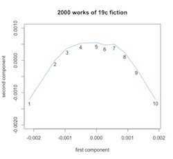
Postscript Jan 5: Have to admit I’ve found it hard to stop exploring this method. I ran it on a fiction dataset expanded to 4,000 works, and to 1922, and patterns started to become a little more legible. For instance, when I include more of her works, George Eliot no longer looks as idiosyncratic. It’s also kind of interesting to superimpose plot arcs for three different periods. Here I’ve borrowed Ben’s idea of using PCA so to speak “out-of-sample,” since each of these periods is actually projected into a different space (defined by the other two periods).

Generalized narrative arcs for 4,000 works of fiction from 1700 to 1922. Very few of them are actually before 1800, though. — Generalized narrative arcs for 4,000 works of fiction from 1700 to 1922. In each case we’re plotting ten composite points representing the topic distributions for segments of narrative time, and time moves from left to right. The dataset does include reprints.

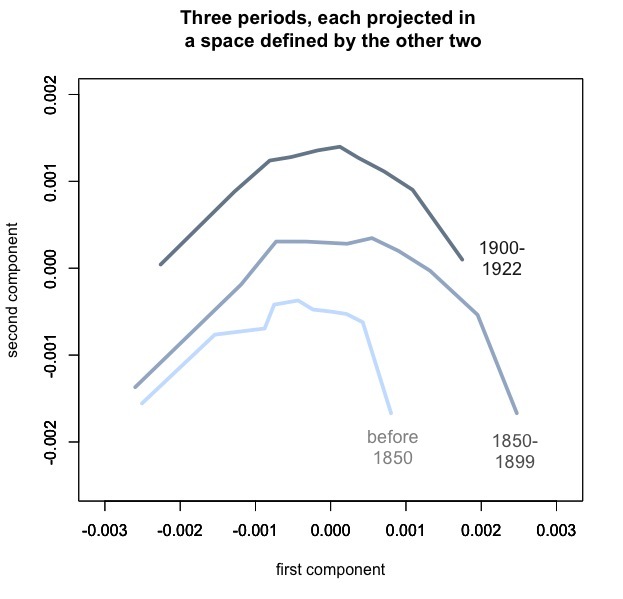
The fact that these arcs float upward may confirm something we already knew, which is that fiction tends to move away from “summary” and toward direct presentation of “scene” as historical time passes. But I think the stability of the pattern is also significant. As Ben has shown, there’s no guarantee that you’ll get an arc if you project a dataset into a PCA space defined by a different dataset. The congruence of these three arcs may not quite prove that plot *is* an arc, but it does suggest that linguistic signals of “beginnings,” “middles,” and “ends” remained broadly similar from the early nineteenth century through the early twentieth. If we wanted to confirm that, we could make more direct comparisons, but for exploratory visualization I see how PCA is useful here.

18c 19c 20c collection-building discovery strategies machine learning

How to find English-language fiction, poetry, and drama in HathiTrust.

Post author By tedunderwood
Post date December 29, 2014

The relative sizes of different genres, represented as a percentage of pages in the English-language portion of HathiTrust. 854,476 volumes are covered. Nonfiction, front matter, and back matter aren't represented here. Results have been smoothed with a five-year moving average.

Although methods of analysis are more fun to discuss, the most challenging part of distant reading may still be locating the texts in the first place [1].

In principle, millions of books are available in digital libraries. But literary historians need collections organized by genre, and locating the fiction or poetry in a digital library is not as simple as it sounds. Older books don’t necessarily have genre information attached. (In HathiTrust, less than 40% of English-language fiction published before 1923 is tagged “fiction” in the appropriate MARC control field.)

Volume-level information wouldn’t be enough to guide machine reading in any case, because genres are mixed up inside volumes. For instance Hoyt Long, Richard So, and I recently published an article in Slate arguing (among other things) that references to specific amounts of money become steadily more common in fiction from 1825 to 1950.

Frequency of reference to "specific amounts" of money in 7,700 English-language works of fiction. Graphics from Wickham, ggplot2 [2]. — Frequency of reference to “specific amounts” of money in 7,700 English-language works of fiction. Graphics here and throughout from Wickham, ggplot2 [2].

But Google’s “English Fiction” collection tells a very different story. The frequencies of many symbols that appear in prices (dollar signs, sixpence) skyrocket in the late nineteenth century, and then drop back by the early twentieth.

Frequencies of "$" and "6d" in Google's "English Fiction" collection, 1800-1950. — Frequencies of “$” and “6d” in Google’s “English Fiction” collection, 1800-1950.

On the other hand, several other words or symbols that tend to appear in advertisements for books follow a suspiciously similar trajectory.

Frequencies of "$", "8vo" (octavo) and "cloth" in Google's "English Fiction" collection, 1800-1950. — Frequencies of “$”, “8vo” (octavo) and “cloth” in Google’s “English Fiction” collection, 1800-1950.

What we see in Google’s “Fiction” collection is something that happens in volumes of fiction, but not exactly in the genre of fiction — the rise and fall of publishers’ catalogs in the backs of books [3]. Individually, these two- or three-page lists of titles for sale may not look like significant noise, but because they often mention prices, and are distributed unevenly across the timeline, they add up to a significant potential pitfall for anyone interested in the role of money in fiction.

I don’t say this to criticize the team behind the Ngram Viewer. Genre wasn’t central to their goals; they provided a rough “fiction” collection merely as a cherry on top of a massively successful public-humanities project. My point is just that genres fail to line up with volume boundaries in ways that can really matter for the questions scholars want to pose. (In fact, fiction may be the genre that comes closest to lining up with volume boundaries: drama and poetry often appear mixed in The Collected Poems and Plays of So-and-So, With a Prose Life of the Author.)

You can solve this problem by selecting works manually, or by borrowing proprietary collections from a vendor. Those are both good, practical solutions, especially up to (say) 1900. But because they rely on received bibliographies, they may not entirely fulfill the promises we’ve been making about dredging the depths of “the great unread,” boldly going where no one has gone before, etc [4]. Over the past two years, with support from the ACLS and NEH, I’ve been trying to develop another alternative — a way of starting with a whole library, and dividing it by genre at the page level, using machine learning.

In researching the Slate article, we relied on that automatic mapping of genre to select pages of fiction from HathiTrust. It helped us avoid conflating advertisements with fiction, and I hope other scholars will also find that it reduces the labor involved in creating large, genre-specific collections. The point of this blog post is to announce the release of a first version of the map we used (covering 854,476 English-language books in HathiTrust 1700-1922).

The whole dataset is available on Figshare, where it has a DOI and is citable as a publication. An interim report is also available; it addresses theoretical questions about genre, as well as questions about methods and data format. And the code we used for the project is available on Github.

For in-depth answers to questions, please consult the interim project report. It’s 47 pages long; it actually explains the project; this blog post doesn’t. But here are a few quick FAQs just so you can decide whether to read further.

“What categories did you try to separate?”

We identify pages as paratext (front matter, back matter, ads), prose nonfiction, poetry (narrative and lyric are grouped together), drama (including verse drama), or prose fiction. The report discusses the rationale for these choices, but other choices would be possible.

“How accurate is this map?”

Since genres are social institutions, questions about accuracy are relative to human dissensus. Our pairs of human readers agreed about the five categories just mentioned for 94.5% of the pages they tagged [5]. Relying on two-out-of-three voting (among other things), we boiled those varying opinions down to a human consensus, and our model agreed with the consensus 93.6% of the time. So this map is nearly as accurate as we might expect crowdsourcing to be. But it covers 276 million pages. For full details, see the confusion matrices in the report. Also, note that we provide ways of adjusting the tradeoff between recall and precision to fit a researcher’s top priority — which could be catching everything that might belong in a genre, or filtering out everything that doesn’t belong. We provide filtered collections of drama, fiction, and poetry for scholars who want to work with datasets that are 97-98% precise.

“You just wrote a blog post admitting that even simple generic boundaries like fiction/nonfiction are blurry and contested. So how can we pretend to stabilize a single map of genre?”

The short answer: we can’t. I don’t expect the genre predictions in this dataset to be more than one resource among many. We’ve also designed this dataset to have a certain amount of flexibility. There are confidence metrics associated with each volume, and users can define their collection of, say, poetry more broadly or narrowly by adjusting the confidence thresholds for inclusion. So even this dataset is not really a single map.

“What about divisions below the page level?”

With the exception of divisions between running headers and body text, we don’t address them. There are certainly a wide range of divisions below the page level that can matter, but we didn’t feel there was much to be gained by trying to solve all those problems at the same time as page-level mapping. In many cases, divisions below the page level are logically a subsequent step.

“How would I actually use this map to find stuff?”

There are three different ways — see “How to use this data?” in the interim report. If you’re working with HathiTrust Research Center, you could use this data to define a workset in their portal. Alternatively, if your research question can be answered with word frequencies, you could download public page-level features from HTRC and align them with our genre predictions on your own machine to produce a dataset of word counts from “only pages that have a 97% probability of being prose fiction,” or what have you. (HTRC hasn’t released feature counts for all the volumes we mapped yet, but they’re about to.) You can also align our predictions directly with HathiTrust zip files, if you have those. The pagealigner module in the utilities subfolder of our Github repo is intended as a handy shortcut for people who use Python; it will work both with HT zip files and HTRC feature files, aligning them with our genre predictions and returning a list of pages zipped with genre codes.

Is this sort of collection really what I need for my project?

Maybe not. There are a lot of books in HathiTrust. But as I admitted in my last post, a medium-sized collection based on bibliographies may be a better starting point for most scholars. Library-based collections include things like reprints, works in translation, juvenile fiction, and so on, that could be viewed as giving a fuller picture of literary culture … or could be viewed as messy complicating factors. I don’t mean to advocate for a library-based approach; I’m just trying to expand the range of alternatives we have available.

“What if I want to find fiction in French books between 1900 and 1970?”

Although we’ve made our code available as a resource, we definitely don’t want to represent it as a “tool” that could simply be pointed at other collections to do the same kind of genre mapping. Much of the work involved in this process is domain-specific (for instance, you have to develop page-level training data in a particular language and period). So this is better characterized as a method than a tool, and the report is probably more important than the repo. I plan to continue expanding the English-language map into the twentieth century (algorithmic mapping of genre may in fact be especially necessary for distant reading behind the veil of copyright). But I don’t personally have plans to expand this map to other languages; I hope someone else will take up that task.

As a reward for reading this far, here’s a visualization of the relative sizes of genres across time, represented as a percentage of pages in the English-language portion of HathiTrust.

The relative sizes of different genres, represented as a percentage of pages in the English-language portion of HathiTrust. 854,476 volumes are covered. Nonfiction, front matter, and back matter aren't represented here. Results have been smoothed with a five-year moving average. — The relative sizes of different genres, represented as a percentage of pages in the English-language portion of HathiTrust. 854,476 volumes are covered. Nonfiction, front matter, and back matter aren’t represented here. Results have been smoothed with a five-year moving average. Click through to enlarge.

The image is discussed at more length in the interim progress report.

Acknowledgments

The blog post above often slips awkwardly into first-person plural, because I’m describing a project that involved a lot of people. Parts of the code involved were written by Michael L. Black and Boris Capitanu. The code also draws on machine learning libraries in Weka and Scikit-Learn [6, 7]. Shawn Ballard organized the process of gathering training data, assisted by Jonathan Cheng, Nicole Moore, Clara Mount, and Lea Potter. The project also depended on collaboration and conversation with a wide range of people at HathiTrust Digital Library, HathiTrust Research Center, and the University of Illinois Library, including but not limited to Loretta Auvil, Timothy Cole, Stephen Downie, Colleen Fallaw, Harriett Green, Myung-Ja Han, Jacob Jett, and Jeremy York. Jana Diesner and David Bamman offered useful advice about machine learning. Essential material support was provided by a Digital Humanities Start-Up Grant from the National Endowment for the Humanities and a Digital Innovation Fellowship from the American Council of Learned Societies. None of these people or agencies should be held responsible for mistakes.

References

[1] Perhaps it goes without saying, since the phrase has now lost its quotation marks, but “distant reading” is Franco Moretti, “Conjectures on World Literature,” New Left Review 1 (2000).

[2] Hadley Wickham, ggplot2: Elegant Graphics for Data Analysis. http: //had.co.nz/ggplot2/book. Springer New York, 2009.

[3] Having mapped advertisements in volumes of fiction, I’m pretty certain that they’re responsible for the spike in dollar signs in Google’s “English Fiction” collection. The collection I mapped overlaps heavily with Google Books, and the number of pages of ads in fiction volumes tracks very closely with the frequency of dollars signs, “8vo,” and so on.

Percentage of pages in mostly-fiction volumes that are ads. Based on a filtered collection of 102,349 mostly-fiction volumes selected from a larger group of 854,476 volumes 1700-1922. Five-year moving average.

[4] “The great unread” comes from Margaret Cohen, The Sentimental Education of the Novel (Princeton NJ: Princeton University Press, 1999), 23.

[5] See the interim report (subsection, “Evaluating Confusion Matrices”) for a fuller description; it gets complicated, because we actually assessed accuracy in terms of the number of words misclassified, although the classification was taking place at a page level.

[6] F. Pedregosa, G. Varoquaux, A. Gramfort, V. Michel, B. Thirion, O. Grisel, M. Blondel, P. Prettenhofer, R. Weiss, V. Dubourg, J. Vanderplas, A. Passos, D. Cournapeau, M. Brucher, M. Perrot, and E. Duchesnay. Scikit-learn: Machine learning in Python. Journal of Machine Learning Research, 12:2825–2830, 2011.

[7] Mark Hall, Eibe Frank, Geoffrey Holmes, Bernhard Pfahringer, Peter Reutemann, and Ian H. Witten. The WEKA data mining software: An update. SIGKDD Explorations, 11(1), 2009.

Tags digital humanities, genre, machine learning

19c Bayesian topic modeling discovery strategies topic modeling

Topic modeling made just simple enough.

Post author By tedunderwood
Post date April 7, 2012
86 Comments on Topic modeling made just simple enough.

Right now, humanists often have to take topic modeling on faith. There are several good posts out there that introduce the principle of the thing (by Matt Jockers, for instance, and Scott Weingart). But it’s a long step up from those posts to the computer-science articles that explain “Latent Dirichlet Allocation” mathematically. My goal in this post is to provide a bridge between those two levels of difficulty.

Computer scientists make LDA seem complicated because they care about proving that their algorithms work. And the proof is indeed brain-squashingly hard. But the practice of topic modeling makes good sense on its own, without proof, and does not require you to spend even a second thinking about “Dirichlet distributions.” When the math is approached in a practical way, I think humanists will find it easy, intuitive, and empowering. This post focuses on LDA as shorthand for a broader family of “probabilistic” techniques. I’m going to ask how they work, what they’re for, and what their limits are.

How does it work? Say we’ve got a collection of documents, and we want to identify underlying “topics” that organize the collection. Assume that each document contains a mixture of different topics. Let’s also assume that a “topic” can be understood as a collection of words that have different probabilities of appearance in passages discussing the topic. One topic might contain many occurrences of “organize,” “committee,” “direct,” and “lead.” Another might contain a lot of “mercury” and “arsenic,” with a few occurrences of “lead.” (Most of the occurrences of “lead” in this second topic, incidentally, are nouns instead of verbs; part of the value of LDA will be that it implicitly sorts out the different contexts/meanings of a written symbol.)

Of course, we can’t directly observe topics; in reality all we have are documents. Topic modeling is a way of extrapolating backward from a collection of documents to infer the discourses (“topics”) that could have generated them. (The notion that documents are produced by discourses rather than authors is alien to common sense, but not alien to literary theory.) Unfortunately, there is no way to infer the topics exactly: there are too many unknowns. But pretend for a moment that we had the problem mostly solved. Suppose we knew which topic produced every word in the collection, except for this one word in document D. The word happens to be “lead,” which we’ll call word type W. How are we going to decide whether this occurrence of W belongs to topic Z?

We can’t know for sure. But one way to guess is to consider two questions. A) How often does “lead” appear in topic Z elsewhere? If “lead” often occurs in discussions of Z, then this instance of “lead” might belong to Z as well. But a word can be common in more than one topic. And we don’t want to assign “lead” to a topic about leadership if this document is mostly about heavy metal contamination. So we also need to consider B) How common is topic Z in the rest of this document?

Here’s what we’ll do. For each possible topic Z, we’ll multiply the frequency of this word type W in Z by the number of other words in document D that already belong to Z. The result will represent the probability that this word came from Z. Here’s the actual formula:

Simple enough. Okay, yes, there are a few Greek letters scattered in there, but they aren’t terribly important. They’re called “hyperparameters” — stop right there! I see you reaching to close that browser tab! — but you can also think of them simply as fudge factors. There’s some chance that this word belongs to topic Z even if it is nowhere else associated with Z; the fudge factors keep that possibility open. The overall emphasis on probability in this technique, of course, is why it’s called probabilistic topic modeling.

Now, suppose that instead of having the problem mostly solved, we had only a wild guess which word belonged to which topic. We could still use the strategy outlined above to improve our guess, by making it more internally consistent. We could go through the collection, word by word, and reassign each word to a topic, guided by the formula above. As we do that, a) words will gradually become more common in topics where they are already common. And also, b) topics will become more common in documents where they are already common. Thus our model will gradually become more consistent as topics focus on specific words and documents. But it can’t ever become perfectly consistent, because words and documents don’t line up in one-to-one fashion. So the tendency for topics to concentrate on particular words and documents will eventually be limited by the actual, messy distribution of words across documents.

That’s how topic modeling works in practice. You assign words to topics randomly and then just keep improving the model, to make your guess more internally consistent, until the model reaches an equilibrium that is as consistent as the collection allows.

What is it for? Topic modeling gives us a way to infer the latent structure behind a collection of documents. In principle, it could work at any scale, but I tend to think human beings are already pretty good at inferring the latent structure in (say) a single writer’s oeuvre. I suspect this technique becomes more useful as we move toward a scale that is too large to fit into human memory.

So far, most of the humanists who have explored topic modeling have been historians, and I suspect that historians and literary scholars will use this technique differently. Generally, historians have tried to assign a single label to each topic. So in mining the Richmond Daily Dispatch, Robert K. Nelson looks at a topic with words like “hundred,” “cotton,” “year,” “dollars,” and “money,” and identifies it as TRADE — plausibly enough. Then he can graph the frequency of the topic as it varies over the print run of the newspaper.

As a literary scholar, I find that I learn more from ambiguous topics than I do from straightforwardly semantic ones. When I run into a topic like “sea,” “ship,” “boat,” “shore,” “vessel,” “water,” I shrug. Yes, some books discuss sea travel more than others do. But I’m more interested in topics like this:

You can tell by looking at the list of words that this is poetry, and plotting the volumes where the topic is prominent confirms the guess.

This topic is prominent in volumes of poetry from 1815 to 1835, especially in poetry by women, including Felicia Hemans, Letitia Landon, and Caroline Norton. Lord Byron is also well represented. It’s not really a “topic,” of course, because these words aren’t linked by a single referent. Rather it’s a discourse or a kind of poetic rhetoric. In part it seems predictably Romantic (“deep bright wild eye”), but less colorful function words like “where” and “when” may reveal just as much about the rhetoric that binds this topic together.

A topic like this one is hard to interpret. But for a literary scholar, that’s a plus. I want this technique to point me toward something I don’t yet understand, and I almost never find that the results are too ambiguous to be useful. The problematic topics are the intuitive ones — the ones that are clearly about war, or seafaring, or trade. I can’t do much with those.

Now, I have to admit that there’s a bit of fine-tuning required up front, before I start getting “meaningfully ambiguous” results. In particular, a standard list of stopwords is rarely adequate. For instance, in topic-modeling fiction I find it useful to get rid of at least the most common personal pronouns, because otherwise the difference between 1st and 3rd person point-of-view becomes a dominant signal that crowds out other interesting phenomena. Personal names also need to be weeded out; otherwise you discover strong, boring connections between every book with a character named “Richard.” This sort of thing is very much a critical judgment call; it’s not a science.

I should also admit that, when you’re modeling fiction, the “author” signal can be very strong. I frequently discover topics that are dominated by a single author, and clearly reflect her unique idiom. This could be a feature or a bug, depending on your interests; I tend to view it as a bug, but I find that the author signal does diffuse more or less automatically as the collection expands.

What are the limits of probabilistic topic modeling? I spent a long time resisting the allure of LDA, because it seemed like a fragile and unnecessarily complicated technique. But I have convinced myself that it’s both effective and less complex than I thought. (Matt Jockers, Travis Brown, Neil Fraistat, and Scott Weingart also deserve credit for convincing me to try it.)

This isn’t to say that we need to use probabilistic techniques for everything we do. LDA and its relatives are valuable exploratory methods, but I’m not sure how much value they will have as evidence. For one thing, they require you to make a series of judgment calls that deeply shape the results you get (from choosing stopwords, to the number of topics produced, to the scope of the collection). The resulting model ends up being tailored in difficult-to-explain ways by a researcher’s preferences. Simpler techniques, like corpus comparison, can answer a question more transparently and persuasively, if the question is already well-formed. (In this sense, I think Ben Schmidt is right to feel that topic modeling wouldn’t be particularly useful for the kinds of comparative questions he likes to pose.)

Moreover, probabilistic techniques have an unholy thirst for memory and processing time. You have to create several different variables for every single word in the corpus. The models I’ve been running, with roughly 2,000 volumes, are getting near the edge of what can be done on an average desktop machine, and commonly take a day. To go any further with this, I’m going to have to beg for computing time. That’s not a problem for me here at Urbana-Champaign (you may recall that we invented HAL), but it will become a problem for humanists at other kinds of institutions.

Probabilistic methods are also less robust than, say, vector-space methods. When I started running LDA, I immediately discovered noise in my collection that had not previously been a problem. Running headers at the tops of pages, in particular, left traces: until I took out those headers, topics were suspiciously sensitive to the titles of volumes. But LDA is sensitive to noise, after all, because it is sensitive to everything else! On the whole, if you’re just fishing for interesting patterns in a large collection of documents, I think probabilistic techniques are the way to go.

Where to go next
The standard implementation of LDA is the one in MALLET. I haven’t used it yet, because I wanted to build my own version, to make sure I understood everything clearly. But MALLET is better. If you want a few examples of complete topic models on collections of 18/19c volumes, I’ve put some models, with R scripts to load them, in my github folder.

If you want to understand the technique more deeply, the first thing to do is to read up on Bayesian statistics. In this post, I gloss over the Bayesian underpinnings of LDA because I think the implementation (using a strategy called Gibbs sampling, which is actually what I described above!) is intuitive enough without them. And this might be all you need! I doubt most humanists will need to go further. But if you do want to tinker with the algorithm, you’ll need to understand Bayesian probability.

David Blei invented LDA, and writes well, so if you want to understand why this technique has “Dirichlet” in its name, his works are the next things to read. I recommend his Introduction to Probabilistic Topic Models. It recently came out in Communications of the ACM, but I think you get a more readable version by going to his publication page (link above) and clicking the pdf link at the top of the page.

Probably the next place to go is “Rethinking LDA: Why Priors Matter,” a really thoughtful article by Hanna Wallach, David Mimno, and Andrew McCallum that explains the “hyperparameters” I glossed over in a more principled way.

Then there are a whole family of techniques related to LDA — Topics Over Time, Dynamic Topic Modeling, Hierarchical LDA, Pachinko Allocation — that one can explore rapidly enough by searching the web. In general, it’s a good idea to approach these skeptically. They all promise to do more than LDA does, but they also add additional assumptions to the model, and humanists are going to need to reflect carefully about which assumptions we actually want to make. I do think humanists will want to modify the LDA algorithm, but it’s probably something we’re going to have to do for ourselves; I’m not convinced that computer scientists understand our problems well enough to do this kind of fine-tuning.