Category: Romantic-era writing

[Edit June 8, 2015: This blog post has been rewritten and updated. See Seven Ways Humanists are Using Computers to Understand Text.]

This post is an outline of discussion topics I’m proposing for a workshop at NASSR2012 (a conference of Romanticists). I’m putting it on the blog since some of the links might be useful for a broader audience.

In the morning I’ll give a few examples of concrete literary results produced by text mining. I’ll start the afternoon workshop by opening two questions for discussion: first, what are the obstacles confronting a literary scholar who might want to experiment with quantitative methods? Second, how do those methods actually work, and what are their limits?

I’ll also invite participants to play around with a collection of 818 works between 1780 and 1859, using an R program I’ve provided for the occasion. Links for these materials are at the end of this post.

I. HOW DIFFICULT IS IT TO GET STARTED?
There are two kinds of obstacles: getting the data you need, and getting the digital skills you need.

1. Is it really necessary to have a large collection of texts?
This is up for debate. But I tend to think the answer is “yes.”

Not because bigger is better, or because “distant reading” is the new hotness. It’s still true that a single passage, perceptively interpreted, may tell us more than a thousand volumes.

But if you want to interpret a single passage, you fortunately already have a wrinkled protein sponge that will do a better job than any computer. Quantitative analysis starts to make things easier only when we start working on a scale where it’s impossible for a human reader to hold everything in memory. Your mileage may vary, but I’d say, more than ten books?

And actually, you need a larger collection than that, because quantitative analysis tends to require context before it becomes meaningful. It doesn’t mean much to say that the word “motion” is common in Wordsworth, for instance, until we know whether “motion” is more common in his works than in other nineteenth-century poets. So yes, text-mining can provide clues that lead to real insights about a single author or text. But it’s likely that you’ll need a collection of several hundred volumes, for comparison, before those clues become legible.

This isn’t to deny that there are interesting things that can be done digitally with a single text: digital editing, building timelines and maps, and so on. I just doubt that quantitative analysis adds much value at that scale. (And to give credit where it’s due: Mark Olsen was saying all this back in the 90s — see References.)

2. So, where do I get all those texts?
That’s what I was asking myself 18 months ago. A lot of excitement about digital humanities is premised on the notion that we already have large collections of digitized sources waiting to be used. But it’s not true, because page images are not the same thing as clean, machine-readable text.

If you’re interested in twentieth-century secondary sources, the JSTOR Data for Research API can probably get you what you need. Primary sources are a harder problem. In our own (Romantic) era, optical character recognition (OCR) is unreliable. The ratio of words transcribed accurately ranges from around 80% to around 98%, depending on print quality and typographical quirks like the notorious “long s.” For a lot of text-mining purposes, 95% might be fine, if the errors were randomly distributed. But they’re not random: errors cluster in certain words and periods.

The problem can be addressed in several different ways. There are a few collections (like ECCO-TCP and the Brown Women Writers Project) that transcribe text manually. That’s an ideal solution, but coverage of that kind is stronger in the eighteenth than the nineteenth century.

So Jordan Sellers and I have supplemented those collections by automatically correcting 19c OCR that we got from the Internet Archive. Our strategy involved statistically cautious, period-specific spellchecking, combined with enough reasoning about context to realize that “mortal fin” is probably “mortal sin,” even though “fin” is a correctly spelled word. It’s not a perfect solution, but in our period it works well enough for text-mining purposes. We have corrected about 2,000 volumes this way, and are happy to share our texts and metadata, as well as the spellchecker itself (once I get it packaged well enough to distribute). I can give you either a zip file containing the 19c texts themselves, or a tab-separated file containing docIDs, words, and word counts for the whole collection. In either scheme, the docIDs are keyed to this metadata file.

Of course, selecting titles for a collection like this raises intractable questions about representativeness. We tried to maximize diversity while also selecting volumes that seemed to have reached a significant audience. But other scholars may have other priorities. I don’t think it would be useful to seek a single right answer about representativeness; instead, I’d like to see multiple scholars building different kinds of collections, making them all public, and building on each other’s work. Then we would be able to test a hypothesis against multiple collections, and see whether the obvious caveats about representativeness actually make a difference in any given instance.

3. Is it necessary to learn how to program?
I’m not going to try to answer that question, because it’s complex and better addressed through discussion.

I will tell a brief story. I went into this gig thinking that I wouldn’t have to do my own programming, since there were already public toolsets for text-mining (Voyant, MONK, MALLET, TAPoR, SEASR) and for visualization (Gephi). I figured I would just use those.

But I rapidly learned otherwise. Tools like MONK and Voyant taught me what was possible, but they weren’t well adapted for managing a very large collection of texts, and didn’t permit me to make my own methodological innovations. When you start trying to do either of those things, you rapidly need “nonstandard parts,” which means that someone in the team has to be able to program.

That doesn’t have to be a daunting prospect, because the programming involved is of a relatively forgiving sort. It’s not easy, but it’s also not professional software development. So if you want to do it yourself, that’s a plausible aspiration. Alternately, if you want to collaborate with someone, you don’t necessarily need to find “a computer scientist.” A graduate student or fellow humanist who can program will do just fine.

If you do want to learn to program, I would recommend starting with either Python or R. Of the two languages, Python is certainly easier. It’s intuitive, and well-documented, and great for working with text. If you expect to use existing tools (like MALLET), and just need some “glue” to connect them to each other, Python is probably the way to go. R is a more specialized and less intuitive language. But it happens to be specialized in some ways that are useful for text mining. In particular, it has built-in statistical functions, and a built-in plotting/graphing capacity. I’ve used it for the sample exercise that accompanies this post. But if you’re learning to program for the first time, Python might be a better all-around choice, and you could in principle extend it to do everything R does. [Later addition: You could do worse than start with The Programming Historian.]

II. WHAT CAN WE ACTUALLY DO WITH QUANTITATIVE METHODS?
What follows is just a list of elements. Interesting research projects tend to combine several of these elementary operations in ad-hoc ways suited to a particular question. The list of elements runs a little long, so let me cut to the chase: the overall theme I’m trying to convey is that you can build complex arguments on a very simple foundation. Yes, at bottom, text mining is often about counting words. But a) words matter and b) they hang together in interesting ways, like individual dabs of paint that together start to form a picture.

So, to return to the original question: what can we do?

1) Categorize documents. You can “categorize” in several different senses.

a) Information retrieval: retrieve documents that match a query. This is what you do every time you use a search engine.

b) (Supervised) classification: a program can learn to correctly distinguish texts by a given author, or learn (with a bit more difficulty) to distinguish poetry from prose, tragedies from history plays, or “gothic novels” from “sensation novels.” (See “Quantitative Formalism,” Pamphlet 1 from the Stanford Literary Lab.) The researcher has to provide examples of different categories, but doesn’t have to specify how to make the distinction: algorithms can learn to recognize a combination of features that is the “fingerprint” of a given category.

c) (Unsupervised) clustering: a program can subdivide a group of documents using general measures of similarity instead of predetermined categories. This may reveal patterns you don’t expect.

All three of these techniques can achieve amazing results armed with what seems like very crude information about the documents they’re categorizing. We know, intuitively, that merely counting words is not enough to distinguish a tragedy from a history play. But our intuitions are simply wrong — see the lit lab pamphlet I cited above. It turns out that there’s an enormous amount of information contained in relative word frequencies, even if you know nothing about sequence or syntax. As you consider other aspects of text mining, it’s useful to keep this intuitive misfire in mind. Relatively simple statistical techniques often characterize discourse a good deal better than our intuitions would predict.

2) Contrast the vocabulary of different corpora. In a way, this reverses the logic of classifying documents (1b). Instead of using features to sort documents into categories, you start with two categories of documents and contrast them to identify distinctive features.

For instance, you can discover which words (or phrases) are overrepresented in one author or genre (relative to, say, the rest of nineteenth-century literature). It can admittedly be a challenge to interpret the results: this is a kind of evidence we aren’t accustomed to yet. But lists of overrepresented words can be a fruitful source of critical leads to pursue in more traditional ways.

Beyond identifying distinctive words and phrases, corpora can be compared using metrics chosen for some more specific reason. It’s difficult to give an exhaustive list – but, for instance, the argument I’ve been making about generic differentiation is based on a kind of corpus comparison. As a general think-piece on the topic, I recommend Ben Schmidt’s blog post arguing that comparison is an underused and underrated tool; Schmidt’s taxonomy of text-mining techniques in that post was a strong influence on the taxonomy I’m offering here.

3) Trace the history of particular features (words or phrases) over time. This could be viewed as a special category of corpus comparison, where you’re comparing corpora segmented on the time axis.

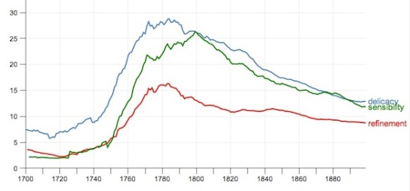
The best-known example here would be Google’s ngram viewer. Digital humanists love to criticize the ngram viewer, partly for valid reasons (there’s no way to know what texts are being used). But it has probably been the single most influential application of text mining, so clearly people are finding this simple kind of diachronic visualization useful. A couple of other projects have built on the same dataset, slicing it in different ways. Mark Davies of BYU built an interface that lets you survey the history of collocations. Our team at Illinois built an interface that mines 18-19c correlations in the ngram dataset; it turns out that correlated words have a high likelihood of being related in other ways as well, and these can be intriguing leads: see what words correlate with “delicacy” in our period, for instance. Harvard has built Bookworm, which can be understood as a smaller but more flexible and better-documented version of the ngram viewer (built on the Open Library instead of Google Books).

Of special interest to Romanticists: a project that isn’t built on the ngram dataset but that does use diachronic correlation-mining as a central methodology. In Stanford Lit Lab Pamphlet 4, Ryan Heuser and Long Le-Khac have traced some very interesting, strongly correlated changes in novelistic diction over the course of the 19th century.

Finally, anyone who wants to make a diachronic argument about diction should read Ben Schmidt’s simple, elegant experiment peeling apart two different components of change: generational succession and historical change within the diction of a single age-cohort.

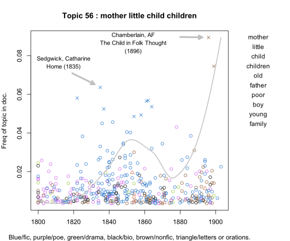
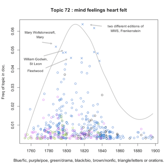
4) Cluster features that tend to be associated in a given corpus of documents (aka topic modeling). In a way, this reverses the logic of clustering documents (1c). Instead of grouping documents that tend to share the same words, you group words that tend to appear in the same documents, or parts of documents. This produces something that looks like a semantic map of the period or corpus you’re studying. (It would be more accurate to call it a discursive map, because topics don’t actually have to be unified semantically. They are more analogous to “discourses.”)

There are a lot of ways to cluster features, ranging from older approaches (Latent Semantic Analysis), to the new, hip approach — “Bayesian topic modeling,” which has the advantage that it clusters individual occurrences of words (tokens) instead of word types. As a result, it can distinguish different senses of a word. (Scott Weingart has written a clear and comprehensive introduction to topic modeling for humanists.)

Topic modeling has become justifiably popular for several reasons. First and foremost, a “discursive map” can be a nice thing to have; it lends itself easily to interpretation. Also, frankly, this approach doesn’t require a whole lot of improvisation. You just pour text files into a tool like MALLET, and out come a list of topics, looking meaningful and authoritative. It’s important to remember that topic-modeling is in fact an imprecise process. Slightly different inputs (for instance, a different stopword list) can produce very different outputs.

5) Entity extraction. If you’re mainly interested in proper nouns (personal names or place names, or dates and prices) there are tools like OpenNLP that can extract these from text, using syntactic patterns as clues.

6) Visualization. Perhaps this isn’t technically a form of analysis, but in practice it’s important enough that it deserves to be treated as a separate analytical step. It’s impractical to list all possible forms of visualization here, but for instance, results can be visualized:

• a) Geographically — to reflect, for instance, density of references to different parts of the world. (See

a quick example of Matt Wilkens’ excellent work

• in this mode — and

a more complete argument available through this conference program.

)

b) As a network graph — to reflect strength of affinity between different entities (characters, or topics, or what have you).

c) Through “Principal Component Analysis,” if you have multidimensional data that need to be flattened to two dimensions for ease of comprehension.

Putting things together.
There’s no limit to the number of ways you can combine these different operations. Matt Wilkens has extracted references to named entities from fiction, and then visualized their density geographically. Robert K. Nelson has performed topic modeling on the print run of a Civil-War-era newspaper, and then graphed the frequency of each topic over time. You could go a step further and look for correlations between topics (either over time, or in terms of their distribution over documents). Then you could visualize the relationships between topics as a network.

What’s the goal uniting all this experimentation? I suspect there are two different but equally valid goals. In some cases, we’re going to find patterns that actually function as evidence to support literary-historical arguments. (In a number of the examples cited above, I think that’s starting to happen.) In other cases, text mining may work mainly as an exploratory technique, revealing clues that need to be fleshed out and written up using more traditional critical methods. The boundary between those two applications will be hotly debated for years, so I won’t attempt to define it here.

III. SAMPLE DATA AND SCRIPT FOR EXPLORATION.
I don’t know whether we’ll really have time for this, but I ought to at least offer you a chance to do hands-on stuff. So here’s a medium-sized project.

I’ve created a pre-packaged set of 818 volumes of poetry and fiction between 1780 and 1859, including 243 authors. I can give you first, a metadata file that includes the authors, titles, dates, and so on for each volume, and second, a data file that includes word counts for each volume. (To keep from frying your laptop, I’ve only included the top 9,000 words in the collection. But actually that’s a lot.)

Finally, I’ve provided an R script that will let you define different chunks of the collection and compare them against each other, to identify words that are significantly overrepresented in a given author, genre, or period. The script will try two different measures of “overrepresentation”: the first, “log-likelihood,” is based on the aggregate frequency of words in the corpus you selected, adding all the volumes in the corpus together. The second, “Mann-Whitney rho,” tries to locate words that are consistently more common in corpus X by paying attention to individual volumes. For more on how that works, see this blog post.

Of course, the R script won’t work until you download R and open it from within R. Please understand that this is a very rough, ad-hoc piece of work for this one occasion, not a polished piece of software that I expect people to use for the long term.

Postscript about the word “mining.”
I know it has an industrial sound; I know humanists like “analysis” more. But I’m sticking with the mining metaphor on the principle of truth in advertising. I think that word accurately conveys the scale of this enterprise, and the fact that it’s often more exploratory than probative. Besides, “mining” is vivid, and that has its own sort of humanistic value.

References (that aren’t already implicit in links)
Mark Olsen, “Signs, Symbols, and Discourses: A New Direction for Computer-Aided Literature Studies” Computers and the Humanities 27 (1993): 309-314.