Categories
18c 19c genre comparison methodology

The differentiation of literary and nonliterary diction, 1700-1900.

When you stumble on an interesting problem, the question arises: do you blog the problem itself — or wait until you have a full solution to publish as an article?

In this case, I think the problem is too big to be solved by a single person anyway, so I might as well get it out there where we can all chip away at it. At the end of this post, I include a link to a page where you can also download the data and code I’m using.

When we compare groups of texts, we’re often interested in characterizing the contrast between them. But instead of characterizing the contrast, you could also just measure the distance between categories. For instance, you could generate a list of word frequencies for two genres, and then run a Spearman’s correlation test, to measure the rank-order similarity of their diction.

In isolation, a measure of similarity between two genres is hard to interpret. But if you run the test repeatedly to compare genres at different points in time, the changes can tell you when the diction of the genres becomes more or less similar.
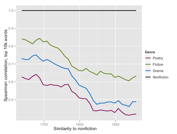
Spearman similarity to nonfiction, measured at 5-year intervals. At each interval, a 39-year chunk of the collection (19 years on either side of the midpoint) is being selected for comparison.

In the graph above, I’ve done that with four genres, in a collection of 3,724 eighteenth- and nineteenth-century volumes (constructed in part by TCP and in part by Jordan Sellers — see acknowledgments), using the 10,000 most frequent words in the collection, excluding proper nouns. The black line at the top is flat, because nonfiction is always similar to itself. But the other lines decline as poetry, drama, and fiction become progressively less similar to nonfiction where word choice is concerned. Unsurprisingly, prose fiction is always more similar to nonfiction than poetry is. But the steady decline in the similarity of all three genres to nonfiction is interesting. Literary histories of this period have tended to pivot on William Wordsworth’s rebellion against a specialized “poetic diction” — a story that would seem to suggest that the diction of 19c poetry should be less different from prose than 18c poetry had been. But that’s not the pattern we’re seeing here: instead it appears that a differentiation was setting in between literary and nonliterary language.

This should be described as a differentiation of “diction” rather than style. To separate style from content (for instance to determine authorship) you need to focus on the frequencies of common words. But when critics discuss “diction,” they’re equally interested, I think, in common and less common words — and that’s the kind of measure of similarity that Spearman’s correlation will give you (Kilgarriff 2001).

The graph above makes it look as though nonfiction was remaining constant while other genres drifted away from it. But we are after all graphing a comparison with two sides. This raises the question: were poetry, fiction, and drama changing relative to nonfiction, or was nonfiction changing relative to them? But of course the answer is “both.”
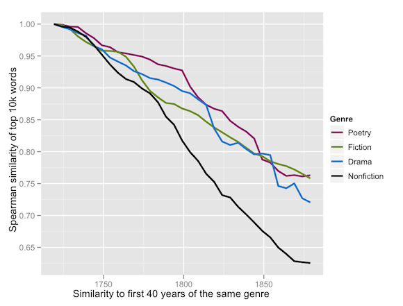
At each 5-year interval, the Spearman similarity is being measured between the 40-year span surrounding that point and the period 1700-1740.

Here we’re comparing each genre to its own past. The language of nonfiction changes somewhat more rapidly than the language of the other genres, but none of them remain constant. There is no fixed reference point in this world, which is why I’m talking about the “differentiation” of two categories. But even granting that, we might want to pose another skeptical question: when literary genres become less like nonfiction, is that merely a sign of some instability in the definition of “nonfiction”? Did it happen mostly because, say, the nineteenth century started to publish on specialized scientific topics? We can address this question to some extent by selecting a more tightly defined subset of nonfiction as a reference point — say, biographies, letters, and orations.
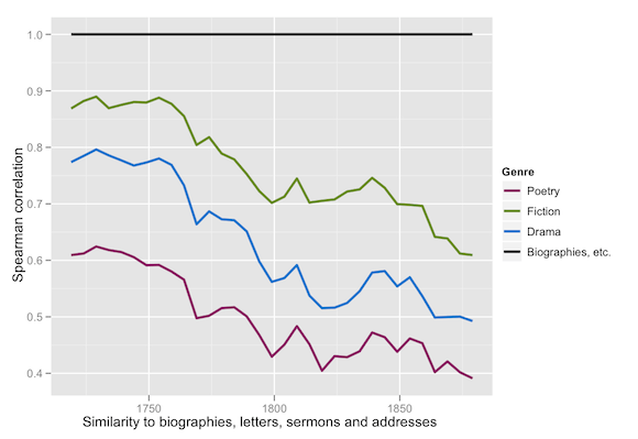
The Spearman similarities here happen to be generated on the top 5000 words rather than the top 10000, but I have tried both wordsets and it makes very little difference.

Even when we focus on this relatively stable category, we see significant differentiation. Two final skeptical questions need addressing before I try to explain what happened. First, I’ve been graphing results so far as solid lines, because our eyes can’t sort out individual data points for four different variables at once. But a numerically savvy reader will want to see some distributions and error bars before assessing the significance of these results. So here are yearly values for fiction. In some cases these are individual works of fiction, though when there are two or more works of fiction in a single year they have been summed and treated as a group. Each year of fiction is being compared against biographies, letters, and orations for 19 years on either side.
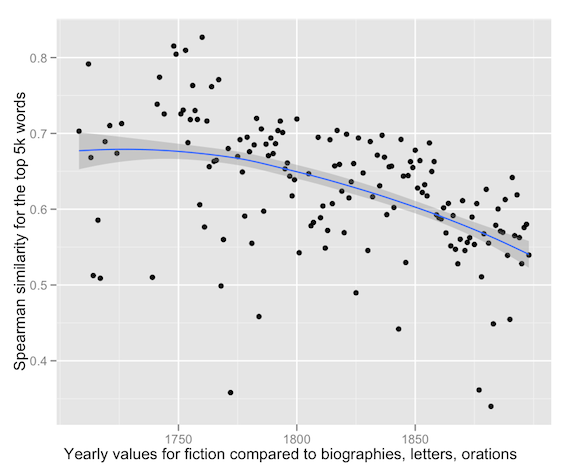
That’s a fairly persuasive trend. You may, however, notice that the Spearman similarities for individual years on this graph are about .1 lower than they were when we graphed fiction as a 39-year moving window. In principle Spearman similarity is independent of corpus size, but it can be affected by the diversity of a corpus. The similarity between two individual texts is generally going to be lower than the similarity between two large and diverse corpora. So could the changes we’ve seen be produced by changes in corpus size? There could be some effect, but I don’t think it’s large enough to explain the phenomenon. [See update at the bottom of this post. The results are in fact even clearer when you keep corpus size constant. -Ed.] The sizes of the corpora for different genres don’t change in a way that would produce the observed decreases in similarity; the fiction corpus, in particular, gets larger as it gets less like nonfiction. Meanwhile, it is at the same time becoming more like poetry. We’re dealing with some factor beyond corpus size.
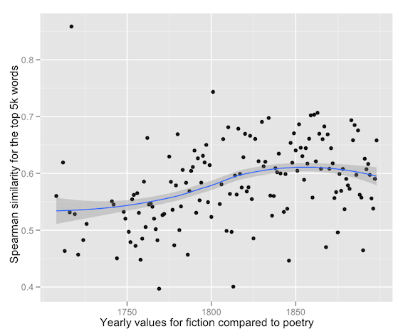
So how then do we explain the differentiation of literary and nonliterary diction? As I started by saying, I don’t expect to provide a complete answer: I’m raising a question. But I can offer a few initial leads. In some ways it’s not surprising that novels would gradually become less like biographies and letters. The novel began very much as faked biography and faked correspondence. Over the course of the period 1700-1900 the novel developed a sharper generic identity, and one might expect it to develop a distinct diction. But the fact that poetry and drama seem to have experienced a similar shift (together with the fact that literary genres don’t seem to have diverged significantly from each other) begins to suggest that we’re looking at the emergence of a distinctively “literary” diction in this period.
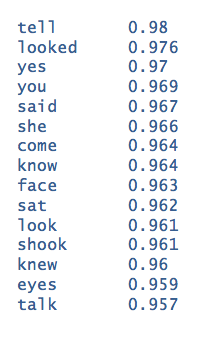
To investigate the character of that diction, we need to compare the vocabulary of genres at many different points. If we just compared late-nineteenth-century fiction to late-nineteenth-century nonfiction, we would get the vocabulary that characterized fiction at that moment, but we wouldn’t know which aspects of it were really new. I’ve done that on the side here, using the Mann-Whitney rho test I described in an earlier post. As you’ll see, the words that distinguish fiction from nonfiction from 1850 to 1900 are essentially a list of pronouns and verbs used to describe personal interaction. But that is true to some extent about fiction in any period. We want to know what aspects of diction had changed.

In other words, we want to find the words that became overrepresented in fiction as fiction was becoming less like nonfiction prose. To find them, I compared fiction to nonfiction at five-year intervals between 1720 and 1880. At each interval I selected a 39-year slice of the collection and ranked words according to the extent to which they were consistently more prominent in fiction than nonfiction (using Mann-Whitney rho). After moving through the whole timeline you end up with a curve for each word that plots the degree to which it is over or under-represented in fiction over time. Then you sort the words to find ones that tend to become more common in fiction as the whole genre becomes less like nonfiction. (Technically, you’re looking for an inverse Pearson’s correlation, over time, between the Mann-Whitney rho for this word and the Spearman’s similarity between genres.) Here’s a list of the top 60 words you find when you do that:


It’s not hard to see that there are a lot of words for emotional conflict here (“horror, courage, confused, eager, anxious, despair, sorrow, dread, agony”). But I would say that emotion is just one aspect of a more general emphasis on subjectivity, ranging from verbs of perception (“listen, listened, watched, seemed, feel, felt”) to explicitly psychological vocabulary (“nerves, mind, unconscious, image, perception”) to questions about the accuracy of perception (“dream, real, sight, blind, forget, forgot, mystery, mistake”). To be sure, there are other kinds of words in the list (“cottage, boy, carriage”). But since we’re looking at a change across a period of 200 years, I’m actually rather stunned by the thematic coherence of the list. For good measure, here are words that became relatively less common in fiction (or more common in nonfiction — that’s the meaning of “relatively”) as the two genres differentiated:
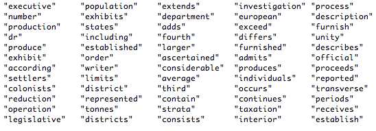

Looking at that list, I’m willing to venture out on a limb and suggest that fiction was specializing in subjectivity while nonfiction was tending to view the world from an increasingly social perspective (“executive, population, colonists, department, european, colonists, settlers, number, individuals, average.”)

Now, I don’t pretend to have solved this whole problem. First of all, the lists I just presented are based on fiction; I haven’t yet assessed whether there’s really a shared “literary diction” that unites fiction with poetry and drama. Jordan and I probably need to build up our collection a bit before we’ll know. Also, the technique I just used to select lists of words looks for correlations across the whole period 1700-1900, so it’s going to select words that have a relatively continuous pattern of change throughout this period. But it’s also entirely possible that “the differentiation of literary and nonliterary diction” was a phenomenon composed of several different, overlapping changes with a smaller “wavelength” on the time axis. So I would say that there’s lots of room here for alternate/additional explanations.

But really, this is a question that does need explanation. Literary scholars may hate the idea of “counting words,” but arguments about a distinctively “literary” language have been central to literary criticism from John Dryden to the Russian Formalists. If we can historicize that phenomenon — if we can show that a systematic distinction between literary and nonliterary language emerged at a particular moment for particular reasons — it’s a result that ought to have significance even for literary scholars who don’t consider themselves digital humanists.

By the way, I think I do know why the results I’m presenting here don’t line up with our received impression that “poetic diction” is an eighteenth-century phenomenon that fades in the 19c. There is a two-part answer. For one thing, part of what we perceive as poetic diction in the 18c is orthography (“o’er”, “silv’ry”). In this collection, I have deliberately normalized orthography, so “silv’ry” is treated as equivalent to “silvery,” and that aspect of “poetic diction” is factored out.

But we may also miss differentiation because we wrongly assume that plain or vivid language cannot be itself a form of specialization. Poetic diction probably did become more accessible in the 19c than it had been in the 18c. But this isn’t the same thing as saying that it became less specialized! A self-consciously plain or restricted diction still counts as a mode of specialization relative to other written genres. More on this in a week or two …

Finally, let me acknowledge that the work I’m doing here is built on a collaborative foundation. Laura Mandell helped me obtain the TCP-ECCO volumes before they were public, and Jordan Sellers selected most of the nineteenth-century collection on which this work is based — something over 1,600 volumes. While Jordan and I were building this collection, we were also in conversation with Loretta Auvil, Boris Capitanu, Tanya Clement, Ryan Heuser, Matt Jockers, Long Le-Khac, Ben Schmidt, and John Unsworth, and were learning from them how to do this whole “text mining” thing. The R/MySQL infrastructure for this is pretty directly modeled on Ben’s. Also, since the work was built on a collaborative foundation, I’m going to try to give back by sharing links to my data and code on this “Open Data” page.

References
Adam Kilgarriff, “Comparing Corpora,” International Journal of Corpus Linguistics 6.1 (2001): 97-133.

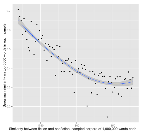
[UPDATE Monday Feb 27th, 7 pm: After reading Ben Schmidt’s comment below, I realized that I really had to normalize corpus size. “Probably not a problem” wasn’t going to cut it. So I wrote a script that samples a million-word corpus for each genre every two years. As long as I was addressing that problem, I figured I would address another one that had been nagging at my conscience. I really ought to be comparing a different wordlist each time I run the comparison. It ought to be the top 5000 words in each pair of corpora that get compared — not the top 5000 words in the collection as a whole.

The first time I ran the improved version I got a cloud of meaningless dots, and for a moment I thought my whole hypothesis about genre had been produced by a ‘loose optical cable.’ Not a good moment. But it was a simple error, and once I fixed it I got results that were actually much clearer than my earlier graphs.

I suppose you could argue that, since document size varies across time, it’s better to select corpora that have a fixed number of documents rather than a fixed word size. I ran the script that way too, and it produces results that are noisier but still unambiguous. The moral of the story is: it’s good to have blog readers who keep you honest and force you to clean up your methodology!]

Categories
18c fiction methodology

MLA talk: just the thesis.

Giving a talk this morning at the MLA. There are two main arguments:

1) The first one will be familiar if you’ve read my blog. I suggest that the boundary between “text mining” and conventional literary research is far fuzzier than people realize. There appears to be a boundary only because literary scholars are pretty unreflective about the way we’re currently using full-text search. I’m going to press this point in detail, because it’s not just a metaphor: to produce a simple but useful topic-modeling algorithm, all you have to do is take a search engine and run it backwards.

2) The second argument is newer; I don’t think I’ve blogged about it yet. I’m going to present topic modeling as a useful bridge between “distant” and “close” reading. I’ve found that I often learn most about a genre by modeling it as part of a larger collection that includes many other genres. In that context, a topic-modeling algorithm can highlight peculiar convergences of themes that characterize the genre relative to its contemporary backdrop.

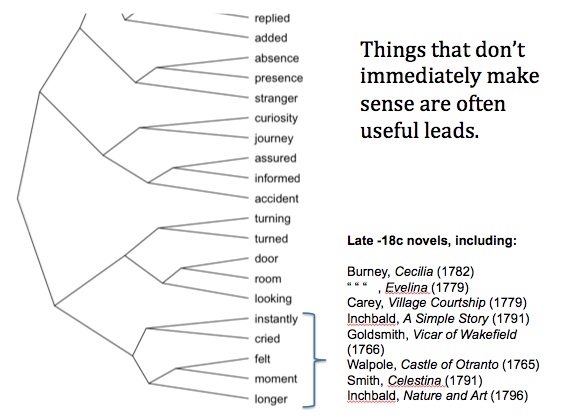
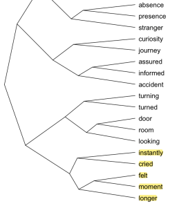
a slide from the talk, where a simple topic-modeling algorithm has been used to produce a dendrogram that offers a clue about the temporal framing of narration in late-18c novels

This is distant reading, in the sense that it requires a large collection. But it’s also close reading, in the sense that it’s designed to reveal subtle formal principles that shape individual works, and that might otherwise elude us.

Although the emphasis is different, a lot of the examples I use are recycled from a talk I gave in August, described here.

Categories
18c 19c math methodology ngrams

Exploring the relationship between topics and trends.

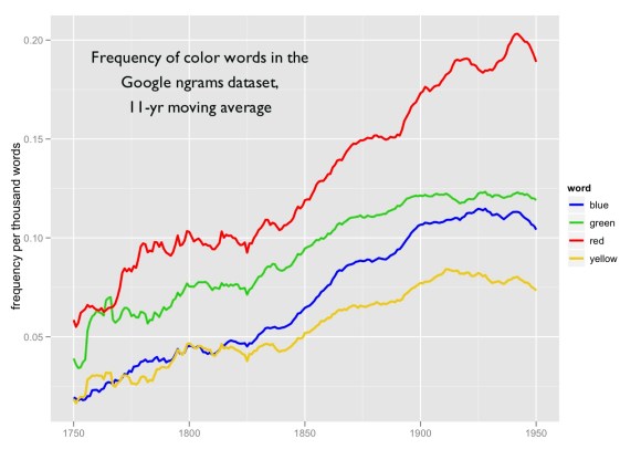
I’ve been talking about correlation since I started this blog. Actually, that was the reason why I did start it: I think literary scholars can get a huge amount of heuristic leverage out of the fact that thematically and socially-related words tend to rise and fall together. It’s a simple observation, and one that stares you in the face as soon as you start to graph word frequencies on the time axis.1 But it happens to be useful for literary historians, because it tends to uncover topics that also pose periodizable kinds of puzzles. Sometimes the puzzle takes the form of a topic we intuitively recognize (say, the concept of “color”) that increases or decreases in prominence for reasons that remain to be explained:

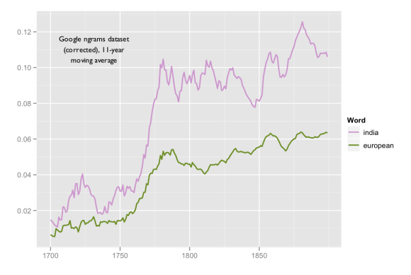
At other times, the connection between elements of the topic is not immediately intuitive, but the terms are related closely enough that their correlation suggests a pattern worthy of further exploration. The relationship between terms may be broadly historical:

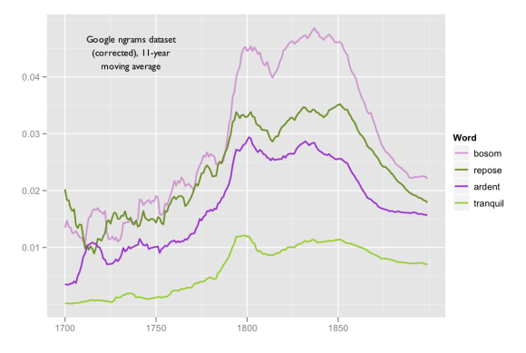
Or it may involve a pattern of expression that characterizes a periodizable style:

Of course, as the semantic relationship between terms becomes less intuitively obvious, scholars are going to wonder whether they’re looking at a real connection or merely an accidental correlation. “Ardent” and “tranquil” seem like opposites; can they really be related as elements of a single discourse? And what’s the relationship to “bosom,” anyway?

Ultimately, questions like this have to be addressed on a case-by-case basis; the significance of the lead has to be fleshed out both with further analysis, and with close reading.

But scholars who are wondering about the heuristic value of correlation may be reassured to know that this sort of lead does generally tend to pan out. Words that correlate with each other across the time axis do in practice tend to appear in the same kinds of volumes. For instance, if you randomly select pairs of words from the top 10,000 words in the Google English ngrams dataset 1700-1849,2 measure their correlation with each other in that dataset across the period 1700-1849, and then measure their tendency to appear in the same volumes in a different collection3 (taking the cosine similarity of term vectors in a term-document matrix), the different measures of association correlate with each other strongly. (Pearson’s r is 0.265, significant at p < 0.0005.) Moreover, the relationship holds (less strongly, but still significantly) even in adjacent centuries: words that appear in the same eighteenth-century volumes still tend to rise and fall together in the nineteenth century.

Why should humanists care about the statistical relationship between two measures of association? It means that correlation-mining is in general going to be a useful way of identifying periodizable discourses. If you find a group of words that correlate with each other strongly, and that seem related at first glance, it's probably going to be worthwhile to follow up the hunch. You’re probably looking at a discourse that is bound together both diachronically (in the sense that the terms rise and fall together) and topically (in the sense that they tend to appear in the same kinds of volumes).

Ultimately, literary historians are going to want to assess correlation within different genres; a dataset like Google's, which mixes all genres in a single pool, is not going to be an ideal tool. However, this is also a domain where size matters, and in that respect, at the moment, the ngrams dataset is very helpful. It becomes even more helpful if you correct some of the errors that vitiate it in the period before 1820. A team of researchers at Illinois and Stanford4, supported by the Andrew W. Mellon Foundation, has been doing that over the course of the last year, and we're now able to make an early version of the tool available on the web. Right now, this ngram viewer only covers the period 1700-1899, but we hope it will be useful for researchers in that period, because it has mostly corrected the long-s problem that confufes opt1cal charader readers in the 18c — as well as a host of other, less notorious problems. Moreover, it allows researchers to mine correlations in the top 10,000 words of the lexicon, instead of trying words one by one to see whether an interesting pattern emerges. In the near future, we hope to expand the correlation miner to cover the twentieth century as well.

For further discussion of the statistical relationship between topics and trends, see this paper submitted to DHCS 2011.

UPDATE Nov 22, 2011: At DHCS 2011, Travis Brown pointed out to me that Topics Over Time (Wang and McCallum) might mine very similar patterns in a more elegant, generative way. I hope to find a way to test that method, and may perhaps try to build an implementation for it myself.

References
1) Ryan Heuser and I both noticed this pattern last winter. Ryan and Long Le-Khac presented on a related topic at DH2011: Heuser, Ryan, and Le-Khac, Long. “Abstract Values in the 19th Century British Novel: Decline and Transformation of a Semantic Field,” Digital Humanities 2011, Stanford University.

2) Jean-Baptiste Michel*, Yuan Kui Shen, Aviva Presser Aiden, Adrian Veres, Matthew K. Gray, William Brockman, The Google Books Team, Joseph P. Pickett, Dale Hoiberg, Dan Clancy, Peter Norvig, Jon Orwant, Steven Pinker, Martin A. Nowak, and Erez Lieberman Aiden*. “Quantitative Analysis of Culture Using Millions of Digitized Books.” Science (Published online ahead of print: 12/16/2010)

3) The collection of 3134 documents (1700-1849) I used for this calculation was produced by combining ECCO-TCP volumes with nineteenth-century volumes selected and digitized by Jordan Sellers.

4) The SEASR Correlation Analysis and Ngrams Viewer was developed by Loretta Auvil and Boris Capitanu at the Illinois Informatics Institute, modeled on prototypes built by Ted Underwood, University of Illinois, and Ryan Heuser, Stanford.

Categories
18c LSA math methodology topic modeling

LSA is a marvellous tool, but literary historians may want to customize it for their own discipline.

Right now Latent Semantic Analysis is the analytical tool I’m finding most useful. By measuring the strength of association between words or groups of words, LSA allows a literary historian to map themes, discourses, and varieties of diction in a given period.

This approach, more than any other I’ve tried, turns up leads that are useful for me as a literary scholar. But when I talk to other people in digital humanities, I rarely hear enthusiasm for it. Why doesn’t LSA get more love? I see three reasons:

1. The word “semantic” is a false lead: it points away from the part of this technique that would actually interest us. It’s true that Latent Semantic Analysis is based on the observation that a word’s distribution across a collection of documents works remarkably well as a first approximation of its meaning. A program running LSA can identify English synonyms on the TOEFL as well as the average student applying to college from a non-English-speaking country. [1]

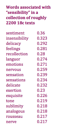
But for a literary historian, the value of this technique does not depend on its claim to identify synonyms and antonyms. We may actually be more interested in contingent associations (e.g., “sensibility” — “rousseau” in the list on the left) than we are in the core “meaning” of a word.

I’ll return in a moment to this point. It has important implications, because it means that we want LSA to do something slightly different than linguists and information scientists have designed it to do. The “flaws” they have tried to iron out of the technique may not always be flaws for our purposes.

2. People who do topic-modeling may feel that they should use more-recently-developed Bayesian methods, which are supposed to be superior on theoretical grounds. I’m acknowledging this point just to set it aside; I’ve mused out loud about it once already, and I don’t want to do more musing until I have rigorously compared the two methods. I will say that from the perspective of someone just getting started, LSA is easier to implement than Bayesian topic modeling: it runs faster and scales up more easily.

3. The LSA algorithm provided by an off-the-shelf package is not necessarily the best algorithm for a literary historian. At bottom, that’s why I’m writing this post: humanists who want to use LSA are going to need guidance from people in their own discipline. Computer scientists do acknowledge that LSA requires “tuning, which is viewed as a kind of art.” [2] But they also offer advice about “best practices,” and some of those best practices are defined by disciplinary goals that humanists don’t share.

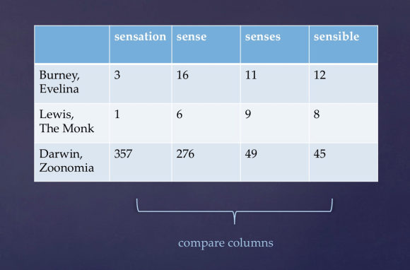
For instance, the power of LSA is often said to come from “reducing the dimensionality of the matrix.” The matrix in question is a term-document matrix — documents are listed along one side of the matrix, and terms along the other, and each cell of the matrix (tfi,j) records the number of times term i appears in document j, modified by a weighting algorithm described at the end of this post.

A (very small) term-document matrix.

That term-document matrix in and of itself can tell you a lot about the associations between words; all you have to do is measure the similarity between the vectors (columns of numbers) associated with each term. But associations of this kind won’t always reveal synonyms. For instance, “gas” and “petrol” might seem unrelated, because they substitute for each other in different sociolects and are rarely found together. To address that problem, you can condense the matrix by factorizing it with a technique called singular value decomposition (SVD). I’m not going to get into the math here, but the key is that condensing the matrix partially fuses related rows and columns — and as a result, the compressed matrix is able to measure transitive kinds of association. The words “gas” and “petrol” may rarely appear together. But they both appear with the same kinds of other words. So when dimensionality reduction “merges” the rows representing similar documents, “gas” and “petrol” will end up being strongly represented in the same merged rows. A compressed matrix is better at identifying synonyms, and for that reason at information retrieval. So there is a lot of consensus among linguists and information scientists that reducing the number of dimensions in the matrix is a good idea.

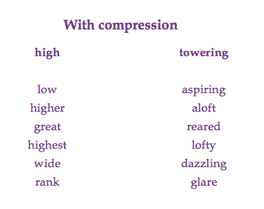
But literary historians approach this technique with a different set of goals. We care a lot about differences of sociolect and register, and may even be more interested in those sources of “noise” than we are in purely semantic relations. “Towering,” for instance, is semantically related to “high.” But I could look that up in a dictionary; I don’t need a computer program to tell me that! I might be more interested to discover that “towering” belongs to a particular subset of poetic diction in the eighteenth century. And that is precisely the kind of accident of distribution that dimensionality-reduction is designed to filter out. For that reason, I don’t think literary applications of LSA are always going to profit from the dimensionality-reduction step that other disciplines recommend.

For about eight months now, I’ve been using a version of LSA without dimensionality reduction. It mines associations simply by comparing the cosine-similarity of term vectors in a term-document matrix (weighted in a special way to address differences of document size). But I wanted to get a bit more clarity about the stakes of that choice, so recently I’ve been comparing it to a version of LSA that does use SVD to compress the matrix.

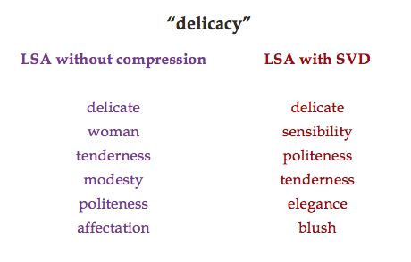
Comparing 18c associations for "delicacy" generated by two different algorithms.

Here’s a quick look at the results. (I’m using 2,193 18c volumes, mostly produced by TCP-ECCO; volumes that run longer than 100,000 words get broken into chunks that can range from 50k-100k words.) In many cases, the differences between LSA with and without compression are not very great. In the case of “delicacy,” for instance, both algorithms indicate that “delicate” has the strongest association. “Politeness” and “tenderness” are also very high on both lists. But compare the second row. The algorithm with compression produces “sensibility” — a close synonym. On the left-hand side, we have “woman.” This is not a synonym for “delicacy,” and if a linguist or computer scientist were evaluating these algorithms, it would probably be rejected as a mistake. But from a literary-historical point of view, it’s no mistake: the association between “delicacy” and femininity is possibly the most interesting fact about the word.
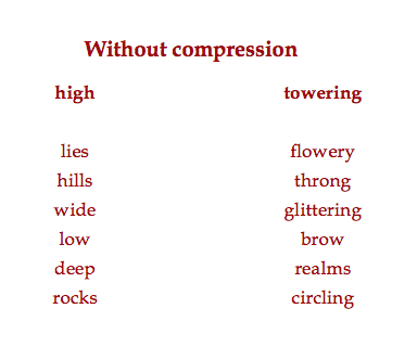
The 18c associations of "high" and "towering," in an uncompressed term-document matrix.

In short, compressing the matrix with SVD highlights semantic relationships at the cost of slightly blurring other kinds of association. In the case of “delicacy,” the effect is fairly subtle, but in other cases the difference between the two approaches is substantial. For instance, if you measure the similarity of term vectors in a matrix without compression, “high” and “towering” look entirely different. The main thing you discover about “high” is that it’s used for physical descriptions of landscape (“lies,” “hills”), and the main thing you discover about “towering” is that it’s used in poetic contexts (“flowery,” “glittering”).
The 18c. associations of "high" and "towering," as measured in a term-document matrix that has undergone SVD compression.

In a matrix that has undergone dimensionality reduction with SVD, associations have a much more semantic character, although they are still colored by other dimensions of context. Which of these two algorithms is more useful for humanistic purposes? I think the answer is going to depend on the goals being pursued in a given research project — if you’re interested in “topics” that are strictly semantic, you might want to use an algorithm that reduces dimensionality with SVD. If you’re interested in discourses, sociolects, genres, or types of diction, you might use LSA without dimensionality reduction.

My purpose here isn’t to choose between those approaches; it’s just to remind humanists that the algorithms we borrow from other disciplines are often going to need to be customized for our own disciplinary purposes. Information scientists have designed topic-modeling algorithms that produce semantically unified topics, because semantic categorization is important for them. But in literary history, we also care about other dimensions of language, and we don’t have to judge topic-modeling algorithms by strictly semantic criteria. How should we judge them? It will probably take decades for us to answer that question fully, but the short answer is just — by how well, in practice, they help us locate critically and historically interesting patterns.

A couple of technical notes: A fine point of LSA that can matter a great deal is how you weight the individual cells in the term-document matrix. For the normal LSA algorithm that uses dimensionality reduction, the consensus is that “log-entropy weighting” works well. You take the log of each frequency, and multiply the whole term vector by the entropy of the vector. I have found that this also works well for humanistic purposes.

For LSA without dimensionality reduction, I would recommend weighting cells by subtracting the expected frequency from the observed frequency. This formula “evens the playing field” between common and uncommon words — and it does so, vitally, in a way that gives a word’s absence from a long document more weight than its absence from a short one. (Much of LSA’s power actually comes from learning where a given word tends not to appear. [3]) I have tried various ways of applying log-entropy weighting without compressing the matrix, and I do not recommend it. Those two techniques belong together.

For reasons that remain somewhat mysterious (although the phenomenon itself is widely discussed), dimensionality reduction seems to work best when the number of dimensions retained is in the range of 250-350. Intuitively, it would seem possible to strike a sort of compromise between LSA methods that do and don’t compress the matrix by reducing dimensionality less drastically (perhaps only, say, cutting it by half). But in practice I find that doesn’t work very well; I suspect compression has to reach a certain threshold before the noise inherent in the process starts to cancel itself out and give way to a new sort of order.

[1] Thomas K. Landauer, Peter W. Foltz, and Darrell Latham, An Introduction to Latent Semantic Analysis, Discourse Processes 25 (1998): 259-84. Web reprint, p. 22.
[2] Preslav Nakov, Elena Valchanova, and Galia Angelova, “Towards Deeper Understanding of Latent Sematic Analysis Performance,” Recent Advances in Natural Language Processing, ed. Nicolas Nicolov (Samokov, Bulgaria: John Benjamins, 2004), 299.
[3] Landauer, Foltz, and Latham, p. 24.

Categories
18c 19c collection-building

The challenges of digital work on early-19c collections.

I’ve been posting mostly about collections built by other people (TCP-ECCO and Google). But I’m also in the process of building a small (thousand-title) 19c collection myself, in collaboration with E. Jordan Sellers. Jordan is selecting titles for the collection; I’m writing the Python scripts that process the texts. This is a modest project intended to support research for a few years, not a model for long-term curatorial practice. But we’ve encountered a few problems specific to the early 19c, and I thought I might share some of our experience and tools in case they’re useful for other early-19c scholars.

Literary and Characteristical Lives (1800), by William and Alexander Smellie. Note esp. the ligatures in 'first' and 'section.'

I originally wanted to create a larger collection, containing twenty or thirty thousand volumes, on the model of Ben Schmidt’s impressive work with nineteenth-century volumes vacuumed up from the Open Library. But because I needed a collection that bridged the eighteenth and nineteenth centuries, I found I had to proceed more slowly. The eighteenth century itself wasn’t the problem. Before 1800, archaic typography makes most optical character recognition unreliable — but for that very reason, TCP-ECCO has been producing clean, manually-keyed versions of 18c texts, enough at least for a small collection. The later 19c also isn’t a problem, because after 1830 or so, OCR quality is mostly adequate.
OCR version of Smellie, contributed by Columbia University Libraries to the Internet Archive.

But between 1800 and (say) 1830, you fall between two stools. It’s technically the nineteenth century, so people assume that OCR ought to work. But in practice, volumes from this period still have a lot of eighteenth-century typographical quirks, including loopy ligatures, the notorious “long s,” and worn or broken type. So the OCR is often pretty vile. I’m willing to put up with background noise if it’s evenly distributed. But these errors are distributed unevenly across the lexicon and across time, so they could actually distort conclusions if left unaddressed.

I decided to build a Python script to do post-processing correction of OCR. There are a lot of ways to do this; my approach was modeled on a paper written by Thomas A. Lasko and Susan E. Hauser for the National Library of Medicine. Briefly, what they show is that OCR correction becomes much more reliable when the program is given statistical information about the language, and errors, to be expected in a given domain. They’re working with contemporary text, but the principle holds even more strongly when you’re working in a different historical period. A generic spellchecker won’t perform well with texts that contain period spellings (“despatch,” “o’erflow’d”), systematic f/s substitution, and a much higher proportion of Latin and French than we’re used to. If your system corrects every occurrence of “même” to “mime,” you’re going to end up with a surprising number of mimes; if you accept “foul” at face value as a correctly-spelled word, you’re going to have very little “soul” in your collection.

Briefly, I customized my spellchecker for the early 19c in three ways:

    • The underlying dictionary included period spellings as well as common French and Latin terms, and recorded the frequency of each term in the 18/19c domain. I used frequencies (lightly) to guide fuzzy matching.
    • To calculate “edit distance,” I used a weighted matrix that recorded the probability of specific character substitutions in early-19c OCR, learning as it went along.
    • To resolve pairs like “foul/soul” and “flip/slip/ship,” where common OCR errors produce a token that could also be a real word, I extracted 2gram frequencies from the Google ngram database so that the program could judge which word made more sense in context. I.e., in the case of “the flip sailed,” the program can infer that a word before “sailed” is pretty likely to be “ship.”

A few other tricks are needed to optimize speed, and to make sure the script doesn’t over-correct proper nouns; anyone who’s interested in doing this should drop me a line for a fuller description and a copy of the code.

Automatically corrected version.

The results aren’t perfect, but they’re good enough to be usable (I am also recording the number of corrections and uncorrectable tokens so that I can assess margins of error later on).

I haven’t packaged this code yet for off-the-shelf use; it’s still got a few trailing wires. But if you want to cannibalize/adapt it, I’d be happy to give you a copy. Perhaps more importantly, I’d like to share a couple of sets of rules that might be helpful for anyone who’s attempting to normalize an 18/19c collection. Both of these rulesets are tab-delimited utf-8 .txt files. First, my list of 4600 rules for correcting 18/19c spellings, including syncopated past-tense forms like “bury’d” and “drop’d.” (Note that syncope cannot always be fixed simply by adding back an “e.” Rules for normalizing poetic syncope — “flow’ry,” “ta’en” — are clustered at the end of the file, so you can delete them if desired.) This ruleset has been transformed by a long series of joins and filtering operations, and edited manually, but I should acknowledge that part of the original list was borrowed from the source files that accompany WordHoard, developed at Northwestern University. I should also warn potential users that these rules are designed to normalize spelling to modern British practice.

The other thing it might be useful to share is a list of 2grams extracted from the Google English corpus, that I use for contextual spellchecking. This includes only 2grams where one of the two elements is a token like “fix” or “flip” that could be read either as a valid word or as an OCR error caused by the long s. Since the long s is also a problem in the Google dataset itself up to 1820, this list was based on frequencies from 1825-50. That’s not perfect for correcting texts in the 1800-1820 period, but I find that in practice it’s adequate. There are two columns here: the 2gram itself, and the frequency.

Categories
18c 19c math ngrams

Words that appear in the same 18c volumes also track each other over time, through the 19c.

I wrote a long post last Friday arguing that topic-modeling an 18c collection is a reliable way of discovering eighteenth- and nineteenth-century trends, even in a different collection.

But when I woke up on Saturday I realized that this result probably didn’t depend on anything special about “topic modeling.” After all, the topic-modeling process I was using was merely a form of clustering. And all the clustering process does is locate the hypothetical centers of more-or-less-evenly-sized clouds of words in vector space. It seemed likely that the specific locations of these centers didn’t matter. The key was the underlying measure of association between words — “cosine similarity in vector space,” which is a fancy way of saying “tendency to be common in the same 18c volumes.” Any group of words that were common (and uncommon) in the same 18c volumes would probably tend to track each other over time, even into the next century.

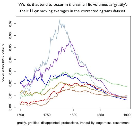
Six words that tend to occur in the same 18c volumes as 'gratify' (in TCP-ECCO), plotted over time in a different collection (a corrected version of Google ngrams).

To test this I wrote a script that chose 200 words at random from the top 5000 in a collection of 2,193 18c volumes (drawn from TCP-ECCO with help from Laura Mandell), and then created a cluster around each word by choosing the 25 words most likely to appear in the same volumes (cosine similarity). Would pairs of words drawn from these randomly distributed clusters also show a tendency to correlate with each other over time?

They absolutely do. The Fisher weighted mean pairwise r for all possible pairs drawn from the same cluster is .267 in the 18c and .284 in the 19c (the 19c results are probably better because Google’s dataset is better in the 19c even after my efforts to clean the 18c up*). At n = 100 (measured over a century), both correlations have rock-solid statistical significance, p < .01. And in case you're wondering … yes, I wrote another script to test randomly selected words using the same statistical procedure, and the mean pairwise r for randomly selected pairs (factoring out, as usual, partial correlation with the larger 5000-word group they’re selected from) is .0008. So I feel confident that the error level here is low.**

What does this mean, concretely? It means that the universe of word-frequency data is not chaotic. Words that appear in the same discursive contexts tend, strongly, to track each other over time, and (although I haven’t tested this rigorously yet), it’s not hard to see that the converse proposition is also going to hold true: words that track each other over time are going to tend to have contextual associations as well.

To put it even more bluntly: pick a word, any word! We are likely to be able to define not just a topic associated with that word, but a discourse — a group of words that are contextually related and that also tend to wax and wane together over time. I don’t imagine that in doing so we prove anything of humanistic significance, but I do think it means that we can raise several thousand significant questions. To start with: what was the deal with eagerness, gratification, and disappointment in the second half of the eighteenth century?

* A better version of Google’s 18c dataset may be forthcoming from the NCSA.

** For people who care about the statistical reliability of data-mining, here’s the real kicker: if you run a Benjamini-Hochberg procedure on these 200 randomly-generated clusters, 134 of them have significance at p < .05 in the 19c even after controlling for the false discovery rate. To put that more intelligibly, these are guaranteed not to be xkcd’s green jelly beans. The coherence of these clusters is even greater than the ones produced by topic-modeling, but that’s probably because they are on average slightly smaller (25 words); I have yet to test the relative importance of different generation procedures while holding cluster size rigorously constant.

Categories
18c 19c math methodology topic modeling trend mining

Topics tend to be trends. Really: p < .05!

While I’m fascinated by cases where the frequencies of two, or ten, or twenty words closely parallel each other, my conscience has also been haunted by a problem with trend-mining — which is that it always works. There are so many words in the English language that you’re guaranteed to find groups of them that correlate, just as you’re guaranteed to find constellations in the night sky. Statisticians call this the problem of “multiple comparisons”; it rests on a fallacy that’s nicely elucidated in this classic xkcd comic about jelly beans.

Simply put: it feels great to find two conceptually related words that correlate over time. But we don’t know whether this is a significant find, unless we also know how many potentially related words don’t correlate.

One way to address this problem is to separate the process of forming hypotheses from the process of testing them. For instance, we could use topic modeling to divide the lexicon up into groups of terms that occur in the same contexts, and then predict that those terms will also correlate with each other over time. In making that prediction, we turn an undefined universe of possible comparisons into a finite set.

Once you create a set of topics, plotting their frequencies is simple enough. But plotting the aggregate frequency of a group of words isn’t the same thing as “discovering a trend,” unless the individual words in the group actually correlate with each other over time. And it’s not self-evident that they will.

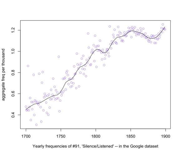
The top 15 words in topic #91, "Silence/Listened," and their cosine similarity to the centroid.

So I decided to test the hypothesis that they would. I used semi-fuzzy clustering to divide one 18c collection (TCP-ECCO) into 200 groups of words that tend to appear in the same volumes, and then tested the coherence of those topics over time in a different 18c collection (a much-cleaned-up version of the Google ngrams dataset I produced in collaboration with Loretta Auvil and Boris Capitanu at the NCSA). Testing hypotheses in a different dataset than the one that generated them is a way of ensuring that we aren’t simply rediscovering the same statistical accidents a second time.

To make a long story short, it turns out that topics have a statistically significant tendency to be trends (at least when you’re working with a century-sized domain). Pairs of words selected from the same topic correlated significantly with each other even after factoring out other sources of correlation*; the Fisher weighted mean r for all possible pairs was 0.223, which measured over a century (n = 100) is significant at p < .05.

In practice, the coherence of different topics varied widely. And of course, any time you test a bunch of hypotheses in a row you're going to get some false positives. So the better way to assess significance is to control for the "false discovery rate." When I did that (using the Benjamini-Hochberg method) I found that 77 out of the 200 topics cohered significantly as trends.

There are a lot of technical details, but I'll defer them to a footnote at the end of this post. What I want to emphasize first is the practical significance of the result for two different kinds of researchers. If you're interested in mining diachronic trends, then it may be useful to know that topic-modeling is a reliable way of discovering trends that have real statistical significance and aren’t just xkcd’s “green jelly beans.”

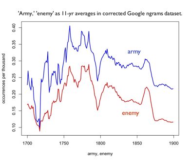
The top 15 terms in topic #89, "Enemy/Attacked," and their cosine similarity to the centroid.

Conversely, if you're interested in topic modeling, it may be useful to know that the topics you generate will often be bound together by correlation over time as well. (In fact, as I’ll suggest in a moment, topics are likely to cohere as trends beyond the temporal boundaries of your collection!)

Finally, I think this result may help explain a phenomenon that Ryan Heuser, Long Le-Khac, and I have all independently noticed: which is that groups of words that correlate over time in a given collection also tend to be semantically related. I've shown above that topic modeling tends to produce diachronically coherent trends. I suspect that the converse proposition is also true: clusters of words linked by correlation over time will turn out to have a statistically significant tendency to appear in the same contexts.

Why are topics and trends so closely related? Well, of course, when you’re topic-modeling a century-long collection, co-occurrence has a diachronic dimension to start with. So the boundaries between topics may already be shaped by change over time. It would be interesting to factor time out of the topic-modeling process, in order to see whether rigorously synchronic topics would still generate diachronic trends.

I haven’t tested that yet, but I have tried another kind of test, to rule out the possibility that we’re simply rediscovering the same trends that generated the topics in the first place. Since the Google dataset is very large, you can also test whether 18c topics continue to cohere as trends in the nineteenth century. As it turns out, they do — and in fact, they cohere slightly more strongly! (In the 19c, 88 out of 200 18c topics cohered significantly as trends.) The improvement is probably a clue that Google’s dataset gets better in the nineteenth century (which god knows, it does) — but even if that’s true, the 19c result would be significant enough on its own to show that topic modeling has considerable predictive power.

Practically, it’s also important to remember that “trends” can play out on a whole range of different temporal scales.

For instance, here’s the trend curve for topic #91, “Silence / Listened,” which is linked to the literature of suspense, and increases rather gradually and steadily from 1700 to the middle of the nineteenth century.

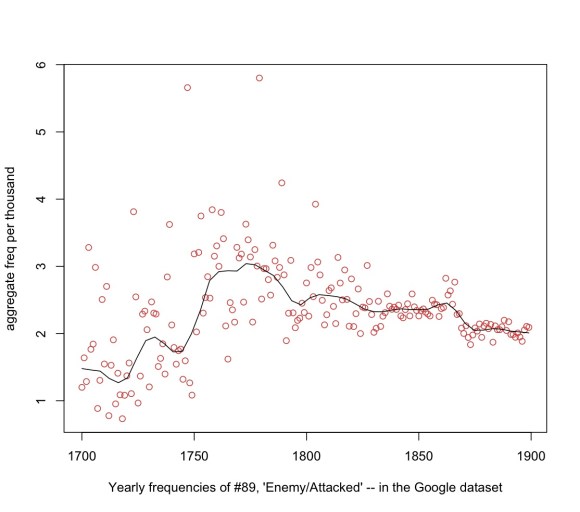
By contrast, here’s the trend curve for topic #89, “Enemy/Attacked,” which is largely used in describing warfare. It doesn’t change frequency markedly from beginning to end; instead it bounces around from decade to decade with a lot of wild outliers. But it is in practice a very tightly-knit trend: a pair of words selected from this topic will have on average 31% of their variance in common. The peaks and outliers are not random noise: they’re echoes of specific armed conflicts.

* Technical details: Instead of using Latent Dirichlet Allocation for topic modeling, I used semi-fuzzy c-means clustering on term vectors, where term vectors are defined in the way I describe in this technical note. I know LDA is the standard technique, and it seems possible that it would perform even better than my clustering algorithm does. But in a sufficiently large collection of documents, I find that a clustering algorithm produces, in practice, very coherent topics, and it has some other advantages that appeal to me. The “semi-fuzzy” character of the algorithm allows terms to belong to more than one cluster, and I use cosine similarity to the centroid to define each term’s “degree of membership” in a topic.

I only topic-modeled the top 5000 words in the TCP-ECCO collection. So in measuring pairwise correlations of terms drawn from the same topic, I had to calculate it as a partial correlation, controlling for the fact that terms drawn from the top 5k of the lexicon are all going to have, on average, a slight correlation with each other simply by virtue of being drawn from that larger group.

Categories
18c 19c fiction methodology

For most literary scholars, text mining is going to be an exploratory tool.

Having just returned from a conference of Romanticists, I’m in a mood to reflect a bit about the relationship between text mining and the broader discipline of literary studies. This entry will be longer than my usual blog post, because I think I’ve got an argument to make that demands a substantial literary example. But you can skip over the example to extract the polemical thesis if you like!

At the conference, I argued that literary critics already practice a crude form of text mining, because we lean heavily on keyword search when we’re tracing the history of a topic or discourse. I suggested that information science can now offer us a wider range of tools for mapping archives — tools that are subtler, more consonant with our historicism, and maybe even more literary than keyword search is.

At the same time, I understand the skepticism that many literary critics feel. Proving a literary thesis with statistical analysis is often like cracking a nut with a jackhammer. You can do it: but the results are not necessarily better than you would get by hand.

One obvious solution would be to use text mining in an exploratory way, to map archives and reveal patterns that a critic could then interpret using nuanced close reading. I’m finding that approach valuable in my own critical practice, and I’d like to share an example of how it works. But I also want to reflect about the social forces that stand in the way of this obvious compromise between digital and mainstream humanists — leading both sides to assume that quantitative analysis ought to contribute instead by proving literary theses with increased certainty.

Part of a topic tree based on a generically diverse collection of 2200 18c texts.

I’ll start with an example. If you don’t believe text mining can lead to literary insights, bear with me: this post starts with some goofy-looking graphs, but develops into an actual hypothesis about the Romantic novel based on normal kinds of literary evidence. But if you’re willing to take my word that text-mining can produce literary leads, or simply aren’t interested in Romantic-era fiction, feel free to skip to the end of this (admittedly long!) post for the generalizations about method.

Several months ago, when I used hierarchical clustering to map eighteenth-century diction on this blog, I pointed to a small section of the resulting tree that intriguingly mixed language about feeling with language about time. It turned out that the words in this section of the tree were represented strongly in late-eighteenth-century novels (novels, for instance, by Frances Burney, Sophia Lee, and Ann Radcliffe). Other sections of the tree, associated with poetry or drama, had a more vivid kind of emotive language, and I wondered why novels would combine an emphasis on feeling or exclamation (“felt,” “cried”) with the abstract topic of duration (“moment,” “longer”). It seemed an oddly phenomenological way to think about emotion.

But I also realized that hierarchical clustering is a fairly crude way of mapping conceptual space in an archive. The preferred approach in digital humanities right now is topic modeling, which does elegantly handle problems like polysemy. However, I’m not convinced that existing methods of topic modeling (LDA and so on) are flexible enough to use for exploration. One of their chief advantages is that they don’t require the human user to make judgment calls: they automatically draw boundaries around discrete “topics.” But for exploratory purposes boundaries are not an advantage! In exploring an archive, the goal is not to eliminate ambiguity so that judgment calls are unnecessary: the goal is to reveal intriguing ambiguities, so that the human user can make judgments about them.

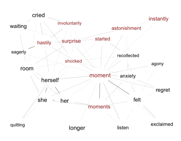
If this is our goal, it’s probably better to map diction as an associative web. Fortunately, it was easy to get from the tree to a web, because the original tree had been based on an algorithm that measured the strength of association between any two words in the collection. Using the same algorithm, I created a list of twenty-five words most strongly associated with the branch that had interested me (“instantly,” “cried,” “felt,” moment,” “longer,”) and then used the strengths of association between those words to model the whole list as a force-directed graph. In this graph, words are connected by “springs” that pull them closer together; the darker the line, the stronger the association between the two words, and the more tightly they will be bound together in the graph. (The sizes of words are loosely proportional to their frequency in the collection, but only very loosely.)

A graph like this is not meant to be definitive: it’s a brainstorming tool that helps me explore associations in a particular collection (here, a generically diverse collection of eighteenth-century writing). On the left side, we see a triangle of feminine pronouns (which are strongly represented in the same novels where “felt,” “moment,” and so on are strongly represented) as well as language that defines domestic space (“quitting,” “room”). On the right side of the graph, we see a range of different kinds of emotion. And yet, looking at the graph as a whole, there is a clear emphasis on an intersection of feeling and time — whether the time at issue is prospective (“eagerly,” “hastily,” “waiting”) or retrospective (“recollected,” “regret”).

In particular, there are a lot of words here that emphasize temporal immediacy, either by naming a small division of time (“moment,” “instantly”), or by defining a kind of immediate emotional response (“surprise,” “shocked,” “involuntarily”). I have highlighted some of these words in red; the decision about which words to include in the group was entirely a human judgment call — which means that it is open to the same kind of debate as any other critical judgment.

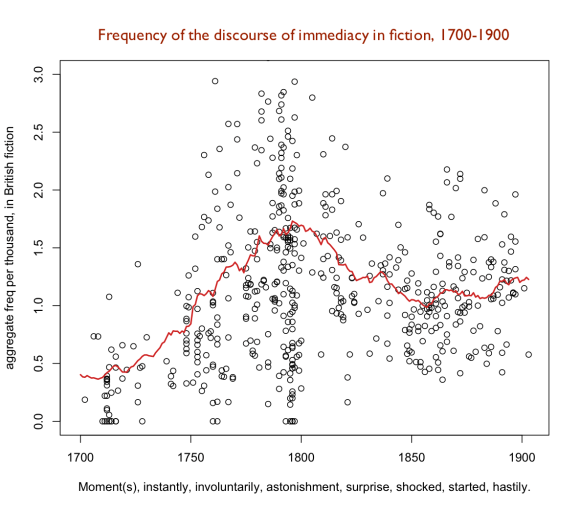
But the group of words I have highlighted in red — let’s call it a discourse of temporal immediacy — does turn out to have an interesting historical profile. We already know that this discourse was common in late-eighteenth-century novels. But we can learn more about its provenance by restricting the generic scope of the collection (to fiction) and expanding its temporal scope to include the nineteenth as well as eighteenth centuries. Here I’ve graphed the aggregate frequency of this group of words in a collection of 538 works of eighteenth- and nineteenth-century fiction, plotted both as individual works and as a moving average. [The moving average won’t necessarily draw a line through the center of the “cloud,” because these works vary greatly in size. For instance, the collection includes about thirty of Hannah More’s “Cheap Repository Tracts,” which are individually quite short, and don’t affect the moving average more than a couple of average-sized novels would, although they create an impressive stack of little circles in the 1790s.]

The shape of the curve here suggests that we’re looking at a discourse that increased steadily in prominence through the eighteenth century and peaked (in fiction) around the year 1800, before sinking back to a level that was still roughly twice its early-eighteenth-century frequency.

Why might this have happened? It’s always a good idea to start by testing the most boring hypothesis — so a first guess might be that words like “moment” and “instantly” were merely displacing some set of close synonyms. But in fact most of the imaginable synonyms for this set of words correlate very closely with them. (This is true, for instance, of words like “sudden,” “abruptly,” and “alarm.”)

Another way to understand what’s going on would be to look at the works where this discourse was most prominent. We might start by focusing on the peak between 1780 and 1820. In this period, the works of fiction where language of temporal immediacy is most prominent include

    Charlotte Dacre, Zofloya (1806)
    Charlotte Lennox, Hermione, or the Orphan Sisters (1791)
    M. G. Lewis, The Monk (1796)
    Ann Radcliffe, A Sicilian Romance (1790), The Castles of Athlin and Dunbayne (1789), and The Romance of the Forest (1792)
    Frances Burney, Cecilia (1782) and The Wanderer (1814)
    Amelia Opie, Adeline Mowbray (1805)
    Sophia Lee, The Recess (1785)

There is a strong emphasis here on the Gothic, but perhaps also, more generally, on women writers. The works of fiction where the same discourse is least prominent would include

    Hannah More, most of her “Cheap Repository Tracts” and Coelebs in Search of a Wife (1809)
    Robert Bage, Hermsprong (1796)
    John Trusler, Life; or the Adventures of William Ramble (1793)
    Maria Edgeworth, Castle Rackrent (1800)
    Arnaud Berquin, The Children’s Friend (1788)
    Isaac Disraeli, Vaurien; or, Sketches of the Times (1797)

Many of these works are deliberately old-fashioned in their approach to narrative form: they are moral parables, or stories for children, or first-person retrospective narratives (like Rackrent), or are told by Fieldingesque narrators who feel free to comment and summarize extensively (as in the works by Disraeli and Trusler).

After looking closely at the way the language of temporal immediacy is used in Frances Burney, Cecilia (1782), and Sophia Lee, The Recess (1785), it seems to me that it had both a formal and an affective purpose.

Formally, it foregrounded a newly sharp kind of temporal framing. If we believe Ian Watt, part of the point of the novel form is to emulate the immediacy of first-hand experience — a purpose that can be slightly at odds with the retrospective character of narrative. Eighteenth-century novelists fought the distancing effect of retrospection in a lot of ways: epistolary narrative, discovered journals and so on are ways of bringing the narrative voice as close as possible to the moment of experience. But those tricks have limits; at some point, if your heroine keeps running off to write breathless letters between every incident, Henry Fielding is going to parody you.

By the late eighteenth century it seems to me novelists were starting to work out ways of combining temporal immediacy with ordinary retrospective narration. Maybe you can’t literally have your narrator describe events as they’re taking place, but you can describe events in a way that highlights their temporal immediacy. This is one of the things that makes Frances Burney read more like a nineteenth-century novelist than like Defoe; she creates a tight temporal frame for each event, and keeps reminding her readers about the tightness of the frame. So, a new paragraph will begin “A few moments after he was gone …” or “At that moment Sir Robert himself burst into the Room …” or “Cecilia protested she would go instantly to Mr Briggs,” to choose a few examples from a single chapter of Cecilia (my italics, 363-71). We might describe this vaguely as a way of heightening suspense — but there are of course many different ways to produce suspense in fiction. Narratology comes closer to the question at issue when it talks about “pacing,” but unless someone has already coined a better term, I think I would prefer to describe this late-18c innovation as a kind of “temporal framing,” because the point is not just that Burney uses “scene” rather than “summary” to make discourse time approximate story time — but that she explicitly divides each “scene” into a succession of discrete moments.

There is a lot more that could be said about this aspect of narrative form. For one thing, in the Romantic era it seems related to a particular way of thinking about emotion — a strategy that heightens emotional intensity by describing experience as if it were divided into a series of instananeous impressions. E.g, “In the cruelest anxiety and trepidation, Cecilia then counted every moment till Delvile came …” (Cecilia, 613). Characters in Gothic fiction are “every moment expecting” some start, shock, or astonishment. “The impression of the moment” is a favorite phrase for both Burney and Sophia Lee. On one page of The Recess, a character “resign[s] himself to the impression of the moment,” although he is surrounded by a “scene, which every following moment threatened to make fatal” (188, my italics).

In short, fairly simple tools for mapping associations between words can turn up clues that point to significant formal, as well as thematic, patterns. Maybe I’m wrong about the historical significance of those patterns, but I’m pretty sure they’re worth arguing about in any case, and I would never have stumbled on them without text mining.

On the other hand, when I develop these clues into a published article, the final argument is likely to be based largely on narratology and on close readings of individual texts, supplemented perhaps by a few simple graphs of the kind I’ve provided above. I suppose I could master cutting-edge natural language processing, in order to build a fabulous tool that would actually measure narrative pace, and the division of scenes into incidents. That would be fun, because I love coding, and it would be impressive, since it would prove that digital techniques can produce literary evidence. But the thing is, I already have an open-source application that can measure those aspects of narrative form, and it runs on inexpensive hardware that requires only water, glucose, and caffeine.

The methodological point I want to make here is that relatively simple forms of text mining, based on word counts, may turn out to be the techniques that are in practice most useful for literary critics. Moreover, if I can speak frankly: what makes this fact hard for us to acknowledge is not technophilia per se, but the nature of the social division between digital humanists and mainstream humanists. Literary critics who want to dismiss text mining are fond of saying “when you get right down to it, it’s just counting words.” (At moments like this we seem to forget everything 20c literary theorists ever learned from linguistics, and go back to treating language as a medium that ideally, ought to be immaterial and transparent. Surely a crudely verbal approach — founded on lumpy, ambiguous words — can never tell us anything about the conceptual subtleties of form and theme!) Stung by that critique, digital humanists often feel we have to prove that our tools can directly characterize familiar literary categories, by doing complex analyses of syntax, form, and sentiment.

I don’t want to rule out those approaches; I’m not interested in playing the game “Computers can never do X.” They probably can do X. But we’re already carrying around blobs of wetware that are pretty good at understanding syntax and sentiment. Wetware is, on the other hand, terrible at counting several hundred thousand words in order to detect statistical clues. And clues matter. So I really want to urge humanists of all stripes to stop imagining that text mining has to prove its worth by proving literary theses.

That should not be our goal. Full-text search engines don’t perform literary analysis at all. Nor do they prove anything. But literary scholars find them indispensable: in fact, I would argue that search engines are at least partly responsible for the historicist turn in recent decades. If we take the same technology used in those engines (a term-document matrix plus vector space math), and just turn the matrix on its side so that it measures the strength of association between terms rather than documents, we will have a new tool that is equally valuable for literary historians. It won’t prove any thesis by itself, but it can uncover a whole new range of literary questions — and that, it seems to me, ought to be the goal of text mining.

References
Frances Burney, Cecilia; or, Memoirs of an Heiress, ed. Peter Sabor and Margaret Ann Doody (Oxford: OUP, 1999).
Sophia Lee, The Recess; or, a Tale of Other Times, ed. April Alliston (Lexington: UP of Kentucky, 2000).

[Postscript: This post, originally titled “How to make text mining serve literary history,” is a version of a talk I gave at NASSR 2011 in Park City, Utah, sharpened by the discussion that took place afterward. I’d like to thank the organizers of the conference (Andrew Franta and Nicholas Mason) as well as my co-panelists (Mark Algee-Hewitt and Mark Schoenfield) and everyone in the audience. The original slides are here; sometimes PowerPoint can be clearer than prose.

I don’t mean to deny, by the way, that the simple tools I’m using could be refined in many ways — e.g., they could include collocations. What I’m saying is I that don’t think we need to wait for technical refinements. Our text-mining tools are already sophisticated enough to produce valuable leads, and even after we make them more sophisticated, it will remain true that at some point in the critical process we have to get off the bicycle and walk.]

Categories
18c 19c visualization

The history of an association, part two.

Here’s another attempt to animate the history of a cluster of associated words — this time as a force-directed graph that folds and unfolds itself as the window of time moves forward, and changing strengths of association create different tensions in the graph.

I had a lot of fun making this clip, but I don’t want to make exaggerated claims for it. These images might not mean very much to me if I hadn’t also read some of the books on which they’re based. The visualization only took a day to build, though, and I think it might turn out to be a useful brainstorming tool. In this instance the clip got me thinking about the different ways time is imagined in the “terror gothic” and in the “horror gothic.”


Association between words is measured here using a vector space model and a collection of more than five hundred works of British fiction. I realize it may seem strange that associations can form and disappear while an eighty-year search window moves forward only sixty years — at the end of this clip the cluster is disappearing while the window still overlaps with the period where the cluster started to emerge. It’s worth recalling that the model isn’t counting words, but measuring the association between them. An early-eighteenth-century work that didn’t use sentimental language at all would do nothing to dilute the association between sentimental terms. But a group of nineteenth-century works that used the same language differently could rapidly obscure earlier patterns.

In short, I suspect that the language of temporal immediacy (“moment,” “suddenly,” “immediately,” and so on) is strongly associated with feeling in the 18c in part because gothic novels, and novels of sensibility, just get to it first. In the nineteenth century other kinds of fiction may take up the same temporal language, diluting its specific connection to tremulous feeling. I can’t prove it yet, but the clues I’m seeing do point in that general direction.

Categories
18c 19c visualization

The history of an association.

[Update May 6th, 2011: The problem I describe here is solved a bit more effectively in a more recent post.] It’s fairly easy to visualize a cluster of associated words. But I’d also like to understand how these associations change, and visualizing that is trickier. For one thing, it’s not easy to define what it means to trace “the same” cluster across time; we need an approach that remains open to the possibility that a particular set of associations could simply weaken or dissolve. The video I’ve embedded below is a first, tentative stab at the problem. Move your mouse pointer away after clicking “play” to see the image without cropping.


I’m trying to understand a late-eighteenth-century convergence between the language of temporality and of feeling. Two words that seemed particularly strongly connected were “moment” and “felt.” So what I’ve done is to proceed five years at a time through a 200-year-long corpus, looking at 80-year-long windows from the corpus. In each “snapshot,” I select the twelve words that associate most strongly in vector space with a vector that’s composed of both “moment” and “felt.” In order to graph them on a coordinate plane, I also measure their association with each term separately. The y axis is association with “moment,” and the x axis is association with “felt.” The reference terms themselves are also plotted. This gives me a way to visualize strength of association in the whole cluster — basically, as everything gets closer to the upper-right-hand corner, the strength of association is getting stronger. At the same time we can get a general sense of the semantic character of the cluster.

I’m working with a relatively small collection here — 538 works of British fiction stretched out between 1700 and 1900. I have a larger 18th-century collection, but in this case I needed continuity over a longer span of time, and in order to achieve that I had to limit the collection to fiction, which reduced its size. It also means that the selection of words you’ll see here is different from the selection of words you saw in previous posts about the “felt-moment” convergence, which were based on a generically diverse collection.

Some of the things that are awkward about this video are consequences of the small collection size. For instance, given the small collection size, I have to choose a pretty long window (80 years out of an overall 200-year-long collection). The window is a bit shorter than that at the beginning of the video — for purely dramatic reasons, so that we don’t reach the “climax” of the clip too rapidly.

Also, of course, the stop-motion animation is rather jerky. With a larger collection, I think it might actually be possible to watch these terms move across the coordinate plane in a smooth and connected fashion. But given the small collection size, smooth motion would be illusory; the data don’t really support that level of precision.

However, even with all those caveats, I feel I’m learning something from the exercise. I think we are glimpsing the transformation of an associative cluster, and looking at the way it changes across time makes me more than ever suspect that — at the moment when it’s strongest — it has something to do with the way late-eighteenth-century fiction imagines suspense. “Anxiety” and “agitation” are durable presences, often in the upper-right-hand corner of the cluster. This interpretation is also, of course, based on reading some of the relevant works, and I think the next stage in exploring the question will be to go back and read them again. As always, I’m inclined to present text-mining more as an exploratory tool or brainstorming technique than as definitive evidence.

It is also a bit interesting to watch the language of gothic agitation turn into language of middle-class striving as we get into the nineteenth century. The intersection between “moment” and “felt” is increasingly occupied not by trembling but by terms like “energy,” “effort,” and “struggle.” I’m not quite sure what to make of that trajectory. Perhaps it helps explain the dissolution of the earlier cluster.

Another way of visualizing clusters like this might be to group terms in a force-directed graph and animate the evolution of the graph across time.