I’ve developed a text-mining strategy that identifies what I call “trending topics” — with apologies to Twitter, where the term is used a little differently. These are diachronic patterns that I find practically useful as a literary historian, although they don’t fit very neatly into existing text-mining categories.
A “topic,” as the term is used in text-mining, is a group of words that occur together in a way that defines a thematic focus. Cameron Blevin’s analysis of Martha Ballard’s diary is often cited as an example: Blevin identifies groups of words that seem to be associated, for instance, with “midwifery,” “death,” or “gardening,” and tracks these topics over the course of the diary.
“Trends” haven’t received as much attention as topics, but we need some way to describe the pattern that Google’s ngram viewer has made so visible, where groups of related words rise and fall together across long periods of time. I suspect “trend” is as a good a name for this phenomenon as we’ll get.
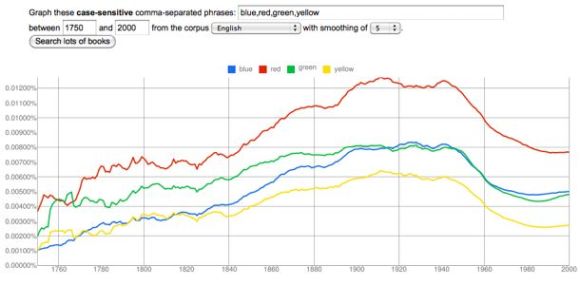
From 1750 to 1920, the prominence of color vocabulary increases by a factor of three, for instance: and when it does, the names of different colors track each other very closely. I would call this a trend. Moreover, it’s possible to extend the principle that conceptually related words rise and fall together beyond cases like the colors and seasons where we’re dealing with an obvious physical category.
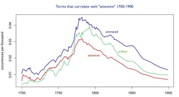
“Animated,” “attentive,” and “ardour” track each other almost as closely as the names of primary colors (the correlation coefficients are around 0.8), and they characterize conduct in ways that are similar enough to suggest that we’re looking at the waxing and waning not just of a few random words, but of a conceptual category — say, a particular sort of interest in states of heightened receptiveness or expressivity.
I think we could learn a lot by thoughtfully considering “trends” of this sort, but it’s also a kind of evidence that’s not easy to interpret, and that could easily be abused. A lot of other words correlate almost as closely with “attentive,” including “propriety,” “elegance,” “sentiments,” “manners,” “flattering,” and “conduct.” Now, I don’t think that’s exactly a random list (these terms could all be characterized loosely as a discourse of manners), but it does cover more conceptual ground than I initially indicated by focusing on words like “animated” and “ardour.” And how do we know that any of these terms actually belonged to the same “discourse”? Perhaps the books that talked about “conduct” were careful not to talk about “ardour”! Isn’t it possible that we have several distinct discourses here that just happened to be rising and falling at the same time?
In order to answer these questions, I’ve been developing a technique that mines “trends” that are at the same time “topics.” In other words, I look for groups of terms that hold together both in the sense that they rise and fall together (correlation across time), and in the sense that they tend to be common in the same documents (co-occurrence). My way of achieving this right now is a two-stage process: first I mine loosely defined trends from the Google ngrams dataset (long lists of, say, one hundred closely correlated words), and then I send those trends to a smaller, generically diverse collection (including everything from sermons to plays) where I can break the list into clusters of terms that tend to occur in the same kinds of documents.
I do this with the same vector space model and hierarchical clustering technique I’ve been using to map eighteenth-century diction on a larger scale. It turns the list of correlated words into a large, branching tree. When you look at a single branch of that tree you’re looking at what I would call a “trending topic” — a topic that represents, not a stable, more-or-less-familiar conceptual category, but a dynamically-linked set of concepts that became prominent at the same time, and in connection with each other.
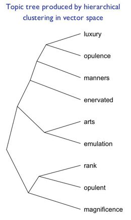
Here, for instance, is a branch of a larger tree that I produced by clustering words that correlate with “manners” in the eighteenth century. It may not immediately look thematically coherent. We might have expected “manners” to be associated with words like “propriety” or “conduct” (which do in fact correlate with it over time), but when we look at terms that change in correlated ways and occur in the same volumes, we get a list of words that are largely about wealth and rank (“luxury,” “opulence,” “magnificence”), as well as the puzzling “enervated.” To understand a phenomenon like this, you can simply reverse the process that generated it, by using the list as a search query in the eighteenth-century collection it’s based on. What turned up in this case were, pre-eminently, a set of mid-eighteenth-century works debating whether modern commercial opulence, and refinements in the arts, have had an enervating effect on British manners and civic virtue. Typical examples are John Brown’s Estimate of the Manners and Principles of the Times (1757) and John Trusler’s Luxury no Political Evil but Demonstratively Proved to be Necessary to the Preservation and Prosperity of States (1781). I was dimly aware of this debate, but didn’t grasp how central it became to debate about manners, and certainly wasn’t familiar with the works by Brown and Trusler.
I feel like this technique is doing what I want it to do, practically, as a literary historian. It makes the ngram viewer something more than a provocative curiosity. If I see an interesting peak in a particular word, I can can map the broader trend of which it’s a part, and then break that trend up into intersecting discourses, or individual works and authors.
Admittedly, there’s something inelegant about the two-stage process I’m using, where I first generate a list of terms and then use a smaller collection to break the list into clusters. When I discussed the process with Ben Schmidt and Miles Efron, they both, independently, suggested that there ought to be some simpler way of distinguishing “trends” from “topics” in a single collection, perhaps by using Principal Component Analysis. I agree about that, and PCA is an intriguing suggestion. On the other hand, the two-stage process is adapted to the two kinds of collections I actually have available at the moment: on the one hand, the Google dataset, which is very large and very good at mapping trends with precision, but devoid of metadata, on the other hand smaller, richer collections that are good at modeling topics, but not large enough to produce smooth trend lines. I’m going to experiment with Principal Component Analysis and see what it can do for me, but in the meantime — speaking as a literary historian rather than a computational linguist — I’m pretty happy with this rough-and-ready way of identifying trending topics. It’s not an analytical tool: it’s just a souped-up search technology that mines trends and identifies groups of works that could help me understand them. But as a humanist, that’s exactly what I want text mining to provide.
Category: 18c
The key to all mythologies.
Well, not really. But it is a classifying scheme that might turn out to be as loopy as Casaubon’s incomplete project in Middlemarch, and I thought I might embrace the comparison to make clear that I welcome skepticism.
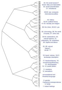
In reality, it’s just a map of eighteenth-century diction. I took the 1,650 most common words in eighteenth-century writing, and asked my iMac to group them into clusters that tend to be common in the same eighteenth-century works. Since the clustering program works recursively, you end up with a gigantic branching tree that reveals how closely words are related to each other in 18c practice. If they appear on the same “branch”; they tend to occur in the same works. If they appear on the same “twig,” that tendency is even stronger.
You wouldn’t necessarily think that two words happening to occur in the same book would tell you much, but when you’re dealing with a large number of documents, it seems there’s a lot of information contained in the differences between them. In any case, this technique produced a detailed map of eighteenth-century topics that seemed — to me, anyway — surprisingly illuminating. To explore a couple of branches, or just marvel at this monument of digital folly, click here, or on the illustration to the right. That’ll take you through to a page where you can click on whichever branches interest you. (Click on the links in the right-hand margin, not the annotations on the tree itself.) To start with, I recommend Branch 18, which is a sort of travel narrative, Branch 13, which is 18c poetic diction in a nutshell, and Branch 5, which is saying something about gender and/or sexuality that I don’t yet understand.
If you want to know exactly how this was produced, and contrast it to other kinds of topic modeling, I describe the technique in this “technical note.” I should also give thanks to the usual cast of characters. Ryan Heuser and Ben Schmidt have produced analogous structures which gave me the idea of attempting this. Laura Mandell and 18th Connect helped me obtain the eighteenth-century texts on which the tree was based.
[UPDATE April 7: The illustrations in this post are now out of date, though some of the explanation may still be useful. The kinds of diction mapped in these illustrations are now mapped better in branches 13-14, 18, and 1 of this larger topic tree.] While trying to understand the question I posed in my last post (why did style become less “conversational” in the 18th century?), I stumbled on a technique that might be useful to other digital humanists. I thought I might pause to describe it.
The technique is basically a kind of topic modeling. But whereas most topic modeling aims to map recurring themes in a single work, this technique maps topics at the corpus level. In other words, it identifies groups of words that are linked by the fact that they tend to occur in the same kinds of books. I’m borrowing this basic idea from Ben Schmidt, who used tf-idf scores to do something similar. I’ve taken a slightly different approach by using a “vector space model,” which I prefer for reasons I’ll describe in some technical notes. But since you’ll need to see results before you care about the how, let me start by showing you what the technique produces.
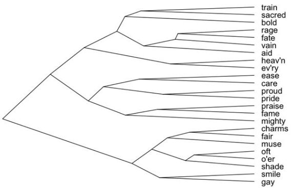
This branch of a larger tree structure was produced by a clustering program that groups words together when they resemble each other according to some measure of similarity. In this case I defined “similarity” as a tendency to occur in the same eighteenth-century texts. Since the tree structure records the sequence of grouping operations, it can register different nested levels of similarity. In the image above, for instance, we can see that “proud” and “pride” are more likely to occur in the same texts than either is to occur together with “smile” or “gay.” But since this is just one branch of a much larger tree, all of these words are actually rather likely to occur together.
This tree is based on a generically diverse collection of 18c texts drawn from ECCO-TCP with help from 18thConnect, and was produced by applying the clustering program I wrote to the 1350 most common words in that collection. The branch shown above represents about 1/50th of the whole tree. But I’ve chosen this branch to start with because it neatly illustrates the underlying principle of association. What do these words have in common? They’re grouped together because they appear in the same kinds of texts, and it’s fairly clear that the “kinds” in this case are poetic. We could sharpen that hypothesis by using this list of words as a search query to see exactly which texts it turns up, but given the prevalence of syncope (“o’er” and “heav’n”), poetry is a safe guess.
It is true that semantically related words tend to be strongly grouped in the tree. Ease/care, charms/fair and so on, are closely linked. But that isn’t a rule built into the algorithm I’m using; the fact that it happens is telling us something about the way words are in practice distributed in the collection. As a result, you get a snapshot of eighteenth century “poetic diction,” not just in the sense of specialized words like “oft,” but in the sense that you can see which themes counted as “poetic” in the eighteenth century, and possibly gather some clues about the way those themes were divided into groups. (In order to find out whether those divisions were generic or historical, you would need to turn the process around and use the sublists as search queries.)
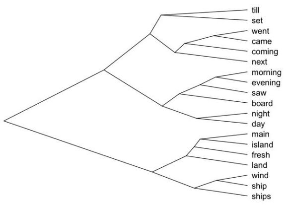
Here’s another part of the tree, showing words that are grouped together because they tend to appear in accounts of travel. The words at the bottom of the image (from “main” to “ships”) are very clearly connected to maritime travel, and the verbs of motion at the top of the image are connected to travel more generally. It’s less obvious that diurnal rhythms like morning/evening and day/night would be described heavily in the same contexts, but apparently they are.
In trees like these, some branches are transparently related to a single genre or subject category, while others are semantically fascinating but difficult to interpret as reflections of a single genre. They may well be produced by the intersection or overlap of several different generic (or historical) categories, and it’ll require more work to understand the nature of the overlap. In a few days I’ll post an overview of the architecture of the whole 1350-word eighteenth-century tree. It’ll be interesting to see how its architecture changes when I slide the collection forward in time to cover progressively later periods (like, say, 1750-1850). But I’m finding the tree interesting for reasons that aren’t limited to big architectural questions of classification: there are interesting thematic clues at every level of the structure. Here’s a portion of one that I constructed with a slightly different list of words.
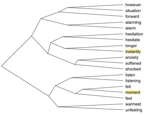
Broadly, I would say that this is the language of sentiment: “alarm,” “softened,” “shocked,” “warmest,” “unfeeling.” But there are also ringers in there, and in a way they’re the most interesting parts. For instance, why are “moment” and “instantly” part of the language of sentiment in the eighteenth century?
William Wordsworth’s claim to have brought poetry back to “the language of conversation in the middle and lower classes of society” gets repeated to each new generation of students (1). But did early nineteenth-century writing in general become more accessible, or closer to speech? It’s hard to say. We’ve used remarks like Wordsworth’s to anchor literary history, but we haven’t had a good way to assess their representativeness.
Increasingly, though, we’re in a position to test some familiar stories about literary history — to describe how the language of one genre changed relative to others, or even relative to “the language of conversation.” We don’t have eighteenth-century English speakers to interview, but we do have evidence about the kinds of words that tend to be more common in spoken language. For instance, Laly Bar-Ilan and Ruth Berman have shown in the journal Linguistics that contemporary spoken English is distinguished from writing by containing a higher proportion of words from the Old English part of the lexicon (2). This isn’t terribly surprising, since English was for a couple of hundred years (1066-1250) almost exclusively a spoken language, while French and Latin were used for writing. Any word that entered English before this period, and survived, had to be the kind of word that gets used in conversation. Words that entered afterward were often borrowed from French or Latin to flesh out the written language.
If the spoken language was distinguished from writing this way in the thirteenth century, and the same thing holds true today, then one might expect it to hold true in the eighteenth and nineteenth centuries as well. And it does seem to hold true: eighteenth-century drama, written to be spoken on stage, is distinguished from nondramatic poetry and prose by containing a higher proportion of Old English words. This is a broad-brush approach to diction, and not one that I would use to describe individual works. But applied to an appropriately large canvas, it may give us a rough picture of how the “register” of written diction has changed across time, becoming more conversational or more formal.
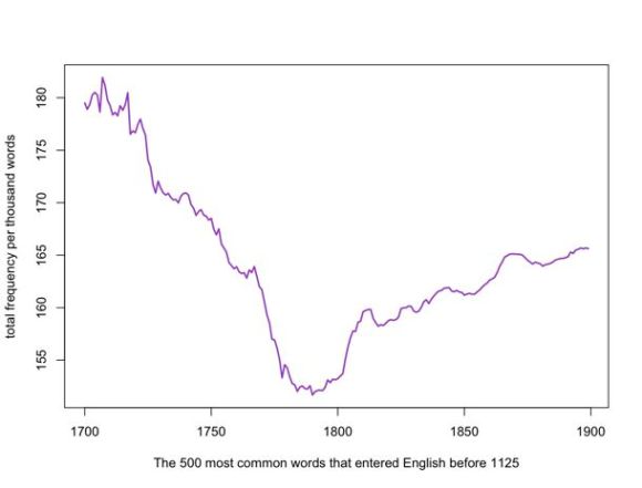
This graph is based on a version of the Google English corpus that I’ve cleaned up in a number of ways. Common OCR errors involving s, f, and ct have been corrected. The graph shows the aggregate frequency of the 500 most common English words that entered the language before the twelfth century. (I’ve found date-of-entry a more useful metric of a word’s affinity with spoken language than terms like “Latinate” or “Germanic.” After all, “Latinate” words like “school,” “street,” and “wall” don’t feel learned to us, because they’ve been transmitted orally for more than a millennium.) I’ve excluded a list of stopwords that includes determiners, prepositions, pronouns, and conjunctions, as well as the auxiliary verbs “be,” “will,” and “have.”
In relative terms, the change here may not look enormous; the peak in the early eighteenth century (181 words per thousand) is only about 20% higher than the trough in the late eighteenth century (152 words per thousand). But we’re talking about some of the most common words in the language (can, think, do, self, way, need, know). It’s a bit surprising that this part of the lexicon fluctuates at all. You might expect to see a gradual decline in the frequency of these words, as the overall size of the lexicon increases. But that’s not what happens: instead we see a rapid decline in the eighteenth century (as prose becomes less like speech, or at least less like the imagined speech of contemporaneous drama), and then a gradual recovery throughout the nineteenth century.
What does this tell us about literature? Not much, without information about genre. After all, as I mentioned, dramatic writing is a lot closer to speech than, say, poetry is. This curve might just be telling us that very few plays got written in the late eighteenth century.
Fortunately it’s possible to check the Google corpus against a smaller corpus of individual texts categorized by genre. I’ve made an initial pass at the first hundred years of this problem using a corpus of 2,188 eighteenth-century books produced by ECCO-TCP, which I obtained in plain text with help from Laura Mandell and 18thConnect. Two thousand books isn’t a huge corpus, especially not after you divide them up by genre, so these results are only preliminary. But the initial results seem to confirm that the change involved the language of prose itself, and not just changes in the relative prominence of different genres. Both fiction and nonfiction prose show a marked change across the century. If I’m right that the frequency of pre-12c words is a fair proxy for resemblance to spoken language, they became less and less like speech.
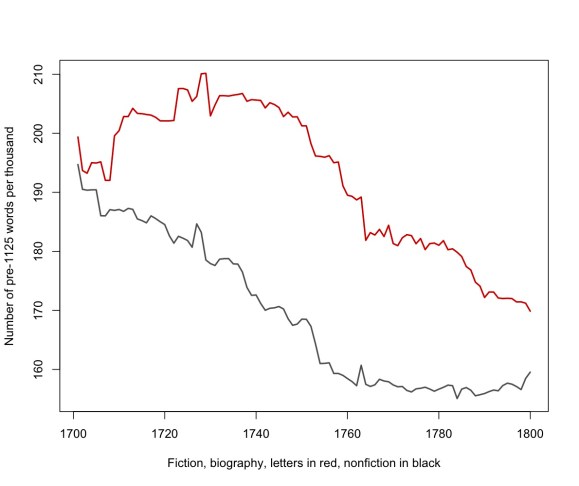
“Fiction” is of course a fuzzy category in the eighteenth century. The blurriness of the boundary between a sensationalized biography and a “novel” is a lot of the point of being a novel. In the graph above, I’ve lumped biographies and collections of personal letters in with novels, because I’m less interested in distinguishing something unique about fiction than I am in confirming a broad change in the diction of nondramatic prose.
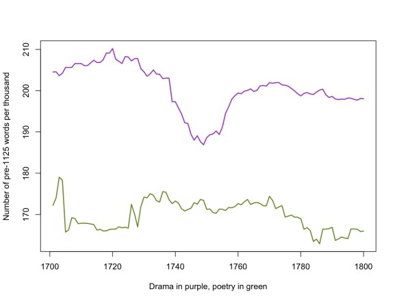
By contrast, there’s relatively little change in the diction of poetry and drama. The proportion of pre-twelfth-century words is roughly the same at the end of the century as it was at the beginning.
Are these results intuitive, or are they telling us something new? I think the general direction of these curves probably confirms some intuitions. Anyone who studies eighteenth and nineteenth-century English knows that you get a lot of long words around 1800. Sad things become melancholy, needs become a necessity, and so on.
What may not be intuitive is how broad and steady the arc of change appears to be. To the extent that we English professors have any explanation for the elegant elaboration of late-eighteenth-century prose, I think we tend to blame Samuel Johnson. But these graphs suggest that much of the change had already taken place by the time Johnson published his Dictionary. Moreover, our existing stories about the history of style put a lot of emphasis on poetry — for instance, on Wordsworth’s critique of poetic diction. But the biggest changes in the eighteenth century seem to have involved prose rather than poetry. It’ll be interesting to see whether that holds true in the nineteenth century as well.
How do we explain these changes? I’m still trying to figure out. In the next couple of weeks I’ll write a post asking what took up the slack: what kinds of language became common in books where old, common words were relatively underrepresented?
—– references —–
1) William Wordsworth and Samuel T. Coleridge, Lyrical Ballads, with a Few Other Poems (Bristol: 1798), i.
2) Laly Bar-Ilan and Ruth A. Berman, “Developing register differentiation: the Latinate-Germanic divide in English,” Linguistics 45 (2007): 1-35.
Until recently, I’ve been limited to working with tools provided by other people. But in the last month or so I realized that it’s easier than it used to be to build these things yourself, so I gave myself a crash course in MySQL and R, with a bit of guidance provided by Ben Schmidt, whose blog Sapping Attention has been a source of many good ideas. I should also credit Matt Jockers and Ryan Heuser at the Stanford Literary Lab, who are doing fabulous work on several different topics; I’m learning more from their example than I can say here, since I don’t want to describe their research in excessive detail.
I’ve now been able to download Google’s 1gram English corpus between 1700 and 1899, and have normalized it to make it more useful for exploring the 18th and 19th centuries. In particular, I normalized case and developed a way to partly correct for the common OCR errors that otherwise make the Google corpus useless in the eighteenth century: especially the substitutions s->f and ss->fl.
Having done that, I built a couple of modules that mine the dataset for patterns. Last December, I was intrigued to discover that words with close semantic relationships tend to track each other closely (using simple sensory examples like the names of colors and oppositions like hot/cold). I suspected that this pattern might extend to more abstract concepts as well, but it’s difficult to explore that hypothesis if you have to test possible instances one by one. The correlation-seeking module has made it possible to explore it more rapidly, and has also put some numbers on what was before a purely visual sense of “fittedness.”
For instance, consider “diction.” It turns out that the closest correlate to “diction” in the period 1700-1899 is “versification,” which has a Pearson correlation coefficient of 0.87. (If this graph doesn’t seem to match the Google version, remember that the ngram viewer is useless in the 18c until you correct for case and long s.)
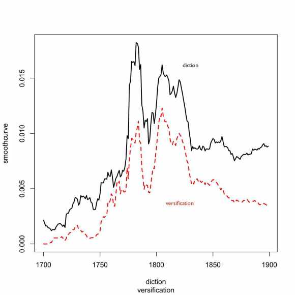
The other words that correlate most closely with “diction” are all similarly drawn from the discourse of poetic criticism. “Poem” and “stanzas” have a coefficient of 0.82; “poetical” is 0.81. It’s a bit surprising that correlation of yearly frequencies should produce such close thematic connections. Obviously, a given subject category will be overrepresented in certain years, and underrepresented in others, so thematically related words will tend to vary together. But in a corpus as large and diverse as Google’s, one might have expected that subtle variation to be swamped by other signals. In practice it isn’t.
I’ve also built a module that looks for words that are overrepresented in a given period relative to the rest of 1700-1899. The measures of overrepresentation I’m using are a bit idiosyncratic. I’m simply comparing the mean frequency inside the period to the mean frequency outside it. I take the natural log of the absolute difference between those means, and multiply it by the ratio (frequency in the period/frequency outside it). For the moment, that formula seems to be working; I’ll try other methods (log-likelihood, etc.) later on.
Once I find a list of, say, fifty words that are overrepresented in a period, I can generate a correlation matrix based on their correlations with each other, and then do hierarchical clustering on that matrix to reveal which words track each other most closely. In effect, I create a broad list of “trending topics” in a particular period, and then use a more precise sort of curve-matching to define the relationships between those trends.
One might imagine that matching words on the basis of change-across-time would be a blunt instrument compared to a more intimate approach based on collocation in the same sentences, or at least co-occurrence in the same volumes. And for many purposes that will be true. But I’ve found that my experiments with smaller-scale co-occurrence (e.g. in MONK) often lead me into tautological dead ends. I’ll discover, e.g., that historical novels share the kind of vocabulary I sort of knew historical novels were likely to share. Relying on yearly frequency data makes it easier to avoid those dead ends, because they have the potential to turn up patterns that aren’t based purely on a single familiar genre or subject category. They may be a blunt instrument, but through their very bluntness they allow us to back up to a vantage point where it’s possible to survey phenomena that are historical rather than purely semantic.
I’ve included an example below. The clusters that emerge here are based on a kind of semantic connection, but often it’s a connection that only makes sense in the context of the period. For instance, “nitrous” and “inflammable” may seem a strange pairing, unless you know that the recently-discovered gas hydrogen was called “inflammable air,” and that chemists were breathing nitrous oxide, aka laughing gas. “Sir” and “de” may seem a strange pairing, unless you reflect that “de” is a French particle of nobility analogous to “sir,” and so on. But I also find that I’m discovering a lot here I didn’t previously know. For instance, I probably should have guessed that Petrarch was a big deal in this period, since there was a sonnet revival — but that’s not something I actually knew, and it took me a while to figure out why Petrarch was coming up. I still don’t know why he’s connected to the dramatist Charles Macklin.
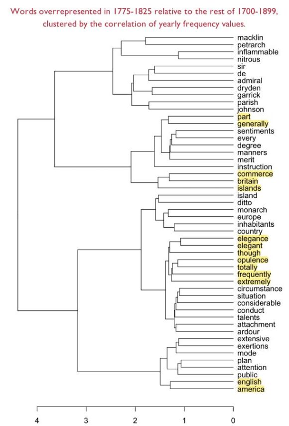
There are lots of other fun pairings in there, especially britain/commerce/islands and the group of flashy hyperbolic adverbs totally/frequently/extremely connected to elegance/opulence. I’m not sure that I would claim a graph like this has much evidentiary value; clustering algorithms are sensitive to slight shifts in initial conditions, so a different list of words might produce different groupings. But I’m also not sure that evidentiary value needs to be our goal. Lately I’ve been inclined to argue that the real utility of text mining may be as a heuristic that helps us discover puzzling questions. I certainly feel that a graph like this helps me identify topics (and more subtly, kinds of periodized diction) that I didn’t recognize before, and that deserve further exploration. [UPDATE 4/20/2011: Back in February I was doing this clustering with yearly frequency data, and Pearson’s correlation, which worked surprisingly well. But I’m now fairly certain that it’s better to do it with co-occurrence data, and a vector space model. See this more recent post.]
It’s only in the last few months that I’ve come to understand how complex search engines actually are. Part of the logic of their success has been to hide the underlying complexity from users. We don’t have to understand how a search engine assigns different statistical weights to different terms; we just keep adding terms until we find what we want. The differences between algorithms (which range widely in complexity, and are based on different assumptions about the relationship between words and documents) never cross our minds.
I’m pretty sure search engines have transformed literary scholarship. There was a time (I can dimly recall) when it was difficult to find new primary sources. You had to browse through a lot of bibliographies looking for an occasional lead. I can also recall the thrill I felt, at some point in the 90s, when I realized that full-text searches in a Chadwyck-Healey database could rapidly produce a much larger number of leads — things relevant to my topic, that no one else seemed to have read. Of course, I wasn’t the only one realizing this. I suspect the wave of challenges to canonical “Romanticism” in the 90s had a lot to do with the fact that Romanticists all realized, around the same time, that we had been looking at the tip of an iceberg.
One could debate whether search engines have exerted, on balance, a positive or negative influence on scholarship. If the old paucity of sources tempted critics to endlessly chew over a small and unrepresentative group of authors, the new abundance may tempt us to treat all works as more or less equivalent — when perhaps they don’t all provide the same kinds of evidence. But no one blames search engines themselves for this, because search isn’t an evidentiary process. It doesn’t claim to prove a thesis. It’s just a heuristic: a technique that helps you find a lead, or get a better grip on a problem, and thus abbreviates the quest for a thesis.
The lesson I would take away from this story is that it’s much easier to transform a discipline when you present a new technique as a heuristic than when you present it as evidence. Of course, common sense tells us that the reverse is true. Heuristics tend to be unimpressive. They’re often quite simple. In fact, that’s the whole point: heuristics abbreviate. They also “don’t really prove anything.” I’m reminded of the chorus of complaints that greeted the Google ngram viewer when it first came out, to the effect that “no one knows what these graphs are supposed to prove.” Perhaps they don’t prove anything. But I find that in practice they’re already guiding my research, by doing a kind of temporal orienteering for me. I might have guessed that “man of fashion” was a buzzword in the late eighteenth century, but I didn’t know that “diction” and “excite” were as well.
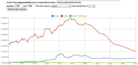
What does a miscellaneous collection of facts about different buzzwords prove? Nothing. But my point is that if you actually want to transform a discipline, sometimes it’s a good idea to prove nothing. Give people a new heuristic, and let them decide what to prove. The discipline will be transformed, and it’s quite possible that no one will even realize how it happened.
POSTSCRIPT, May 1, 2011: For a slightly different perspective on this issue, see Ben Schmidt’s distinction between “assisted reading” and “text mining.” My own thinking about this issue was originally shaped by Schmidt’s observations, but on re-reading his post I realize that we’re putting the emphasis in slightly different places. He suggests that digital tools will be most appealing to humanists if they resemble, or facilitate, familiar kinds of textual encounter. While I don’t disagree, I would like to imagine that humanists will turn out in the end to be a little more flexible: I’m emphasizing the “heuristic” nature of both search engines and the ngram viewer in order to suggest that the key to the success of both lies in the way they empower the user. But — as the word “tricked” in the title is meant to imply — empowerment isn’t the same thing as self-determination. To achieve that, we need to reflect self-consciously on the heuristics we use. Which means that we need to realize we’re already doing text mining, and consider building more appropriate tools.
This post was originally titled “Why Search Was the Killer App in Text-Mining.”
Benjamin Schmidt has been posting some fascinating reflections on different ways of analyzing texts digitally and characterizing the affinities between them.
I’m tempted to briefly comment on a technique of his that I find very promising. This is something that I don’t yet have the tools to put into practice myself, and perhaps I shouldn’t comment until I do. But I’m just finding the technique too intriguing to resist speculating about what might be done with it.
Basically, Schmidt describes a way of mapping the relationships between terms in a particular archive. He starts with a word like “evolution,” identifies texts in his archive that use the word, and then uses tf-idf weighting to identify the other words that, statistically, do most to characterize those texts.
After iterating this process a few times, he has a list of something like 100 terms that are related to “evolution” in the sense that this whole group of terms tends, not just to occur in the same kinds of books, but to be statistically prominent in them. He then uses a range of different clustering algorithms to break this list into subsets. There is, for instance, one group of terms that’s clearly related to social applications of evolution, another that seems to be drawn from anatomy, and so on. Schmidt characterizes this as a process that maps different “discourses.” I’m particularly interested in his decision not to attempt topic modeling in the strict sense, because it echoes my own hesitation about that technique:
In the language of text analysis, of course, I’m drifting towards not discourses, but a simple form of topic modeling. But I’m trying to only submerge myself slowly into that pool, because I don’t know how well fully machine-categorized topics will help researchers who already know their fields. Generally, we’re interested in heavily supervised models on locally chosen groups of texts.
This makes a lot of sense to me. I’m not sure that I would want a tool that performed pure “topic modeling” from the ground up — because in a sense, the better that tool performed, the more it might replicate the implicit processing and clustering of a human reader, and I already have one of those.
Schmidt’s technique is interesting to me because the initial seed word gives it what you might call a bias, as well as a focus. The clusters he produces aren’t necessarily the same clusters that would emerge if you tried to map the latent topics of his whole archive from the ground up. Instead, he’s producing a map of the semantic space surrounding “evolution,” as seen from the perspective of that term. He offers this less as a finished product than as an example of a heuristic that humanists might use for any keyword that interested them, much in the way we’re now accustomed to using simple search strategies. Presumably it would also be possible to move from the semantic clusters he generates to a list of the documents they characterize.
I think this is a great idea, and I would add only that it could be adapted for a number of other purposes. Instead of starting with a particular seed word, you might start with a list of terms that happen to be prominent in a particular period or genre, and then use Schmidt’s technique of clustering based on tf-idf correlations to analyze the list. “Prominence” can be defined in a lot of different ways, but I’m particularly interested in words that display a similar profile of change across time.
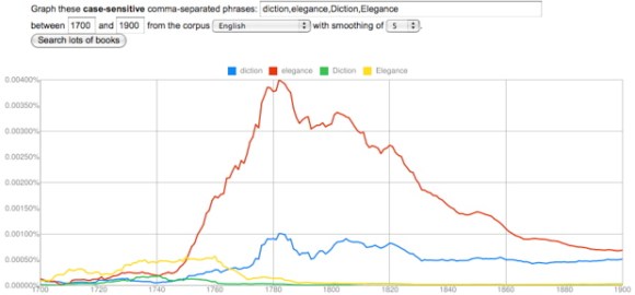
For instance, I think it’s potentially rather illuminating that “diction” and “elegance” change in closely correlated ways in the late eighteenth and early nineteenth century. It’s interesting that they peak at the same time, and I might even be willing to say that the dip they both display, in the radical decade of the 1790s, suggests that they had a similar kind of social significance. But of course there will be dozens of other terms (and perhaps thousands of phrases) that also correlate with this profile of change, and the Google dataset won’t do anything to tell us whether they actually occurred in the same sorts of books. This could be a case of unrelated genres that happened to have emerged at the same time.
But I think a list of chronologically correlated terms could tell you a lot if you then took it to an archive with metadata, where Schmidt’s technique of tf-idf clustering could be used to break the list apart into subsets of terms that actually did occur in the same groups of works. In effect this would be a kind of topic modeling, but it would be topic modeling combined with a filter that selects for a particular kind of historical “topicality” or timeliness. I think this might tell me a lot, for instance, about the social factors shaping the late-eighteenth-century vogue for characterizing writing based on its “diction” — a vogue that, incidentally, has a loose relationship to data mining itself.
I’m not sure whether other humanists would accept this kind of technique as evidence. Schmidt has some shrewd comments on the difference between data mining and assisted reading, and he’s right that humanists are usually going to prefer the latter. Plus, the same “bias” that makes a technique like this useful dispels any illusion that it is a purely objective or self-generating pattern. It’s clearly a tool used to slice an archive from a particular angle, for particular reasons.
But whether I could use it as evidence or not, a technique like this would be heuristically priceless: it would give me a way of identifying topics that peculiarly characterize a period — or perhaps even, as the dip in the 1790s hints, a particular impulse in that period — and I think it would often turn up patterns that are entirely unexpected. It might generate these patterns by looking for correlations between words, but it would then be fairly easy to turn lists of correlated words into lists of works, and investigate those in more traditionally humanistic ways.
For instance, I had no idea that “diction” would correlate with “elegance” until I stumbled on the connection, but having played around with the terms a bit in MONK, I’m already getting a sense that the terms are related not just through literary criticism (as you might expect), but also through historical discourse and (oddly) discourse about the physiology of sensation. I don’t have a tool yet that can really perform Schmidt’s sort of tf-idf clustering, but just to leave you with a sense of the interesting patterns I’m glimpsing, here’s a word cloud I generated in MONK by contrasting eighteenth-century works that contain “elegance” to the larger reference set of all eighteenth-century works. The cloud is based on Dunning’s log likelihood, and limited to adjectives, frankly, just because they’re easier to interpret at first glance.

There’s a pretty clear contrast here between aesthetic and moral discourse, which is interesting to begin with. But it’s also a bit interesting that the emphasis on aesthetics extends into physiological terms like “sensorial,” “irritative,” and “numb,” and historical terms like “Greek” and “Latin.” Moreover, many of the same terms reoccur if you pursue the same strategy with “diction.”
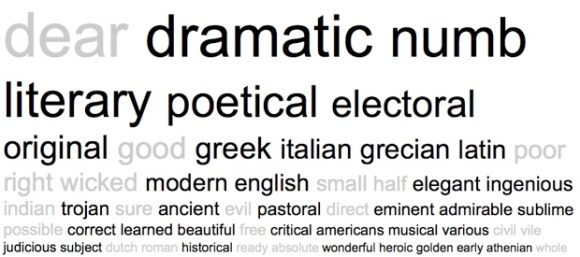
A lot of words here are predictably literary, but again you see sensory terms like “numb,” and historical ones like “Greek,” “Latin,” and “historical” itself. Once again, moreover, moral discourse is interestingly underrepresented. This is actually just one piece of the larger pattern you might generate if you pursued Schmidt’s clustering strategy — plus, Dunning’s is not the same thing as tf-idf clustering, and the MONK corpus of 1000 eighteenth-century works is smaller than one would wish — but the patterns I’m glimpsing are interesting enough to suggest to me that this general kind of approach could tell me a lot of things I don’t yet know about a period.
